6 Effect Sizes
Effect sizes are an important statistical outcome in most empirical studies. Researchers want to know whether an intervention or experimental manipulation has an effect greater than zero, or (when it is obvious that an effect exists) how big the effect is. Researchers are often reminded to report effect sizes, because they are useful for three reasons. First, they allow you to present the magnitude of the reported effects, which in turn allows you to reflect on the practical significance of the effects, in addition to the statistical significance. Second, effect sizes allow researchers to draw meta-analytic conclusions by comparing standardized effect sizes across studies. Third, effect sizes from previous studies can be used when planning a new study in an a-priori power analysis.
A measure of effect size is a quantitative description of the strength of a phenomenon. It is expressed as a number on a scale. For unstandardized effect sizes, the effect size is expressed on the scale that the measure was collected on. This is useful whenever people are able to intuitively interpret differences on a measurement scale. For example, children grow on average 6 centimeters a year between the age of 2 and puberty. We can interpret 6 centimeters a year as an effect size, and many people in the world have an intuitive understanding of how large 6 cm is. Whereas a p-value is used to make a claim about whether there is an effect, or whether we might just be looking at random variation in the data, an effect size is used to answer the question of how large the effect is. This makes an effect size estimate an important complement to p-values in most studies. A p-value tells us that we can claim that children grow as they age; effect sizes tell us what size clothes we can expect children to wear when they are a certain age, and how long it will take before their new clothes are too small.
For people in parts of the world that do not use the metric system, it might be difficult to understand what a difference of 6 cm is. Similarly, a psychologist who is used to seeing scores of 0–20 on their preferred measure of depression might not be able to grasp what a change of 3 points means on a different measure, which could have a scale of 0–10 or 0–50. To facilitate a comparison of effect sizes across situations where different measurement scales are used, researchers can report standardized effect sizes. A standardized effect size, such as Cohen’s d, is computed by dividing the difference on the raw scale by the standard deviation, and is thus scaled in terms of the variability of the sample from which it was taken. An effect of d = 0.5 means that the difference is the size of half a standard deviation of the measure. This means that standardized effect sizes are determined both by the magnitude of the observed phenomenon and the size of the standard deviation. As standardized effect sizes are a ratio of the mean difference divided by the standard deviation, different standardized effect sizes can indicate the mean difference is not identical, or the standard deviations are not identical, or both. It is possible that two studies find the same unstandardized difference, such as a 0.5-point difference on a 7-point scale, but because the standard deviation is larger in Study A (e.g., SD = 2) than in Study B (e.g., SD = 1) the standardized effect sizes differ (e.g., Study 1: 0.5/2 = 0.25, Study B: 0.5/1 = 0.5).
Standardized effect sizes are common when variables are not measured on a scale that people are familiar with, or are measured on different scales within the same research area. If you ask people how happy they are, an answer of ‘5’ will mean something very different if you ask them to answer on a scale from 1 to 5 versus a scale from 1 to 9. Standardized effect sizes can be understood and compared regardless of the scale that was used to measure the dependent variable. Despite the ease of use of standardized effect size measures, there are good arguments to prefer to report and interpret unstandardized effect sizes over standardized effect sizes wherever possible (Baguley, 2009).
Standardized effect sizes can be grouped in two families (Rosnow & Rosenthal (2009)): The d family (consisting of standardized mean differences) and the r family (consisting of measures of strength of association). Conceptually, the d family effect sizes are based on the difference between observations, divided by the standard deviation of these observations, while the r family effect sizes describe the proportion of variance that is explained by group membership. For example, a correlation (\(r\)) of 0.5 indicates that 25% of the variance (\(r^2\)) in the outcome variable is explained by the difference between groups. These effect sizes are calculated from the sum of squares of the residuals (the differences between individual observations and the mean for the group, squared and summed) for the effect, divided by the total sum of squares in the design.
6.1 Effect sizes
What is the most important outcome of an empirical study? You might be tempted to say it’s the p-value of the statistical test, given that it is almost always reported in articles, and determines whether we call something ‘significant’ or not. However, as Cohen (1990) writes in his ‘Things I’ve learned (so far)’:
I have learned and taught that the primary product of a research inquiry is one or more measures of effect size, not p-values.
Although what you want to learn from your data is different in every study, and there is rarely any single thing that you always want to know, effect sizes are a very important part of the information we gain from data collection.
One reason to report effect sizes is to facilitate future research. It is possible to perform a meta-analysis or a power analysis based on unstandardized effect sizes and their standard deviation, but it is easier to work with standardized effect sizes, especially when there is variation in the measures that researchers use. But the main goal of reporting effect sizes is to reflect on the question whether the observed effect size is meaningful. For example, we might be able to reliably measure that, on average, 19-year-olds will grow 1 centimeter in the next year. This difference would be statistically significant in a large enough sample, but if you go shopping for clothes when you are 19 years old, it is not something you need care about. Let’s look at two examples of studies where looking at the effect size, in addition to its statistical significance, would have improved the statistical inferences.
6.2 The Facebook experiment
In the summer of 2014 there were some concerns about an experiment that Facebook had performed on its users to examine ‘emotional mood contagion’, or the idea that people’s moods can be influenced by the mood of people around them. You can read the article here. For starters, there was substantial concern about the ethical aspects of the study, primarily because the researchers who performed the study had not asked for informed consent from the participants in the study, nor did they ask for permission from the institutional review board (or ethics committee) of their university.
One of the other criticisms of the study was that it could be dangerous to influence people’s mood. As Nancy J. Smyth, dean of the University of Buffalo’s School of Social Work wrote on her Social Work blog: “There might even have been increased self-harm episodes, out of control anger, or dare I say it, suicide attempts or suicides that resulted from the experimental manipulation. Did this experiment create harm? The problem is, we will never know, because the protections for human subjects were never put into place”.
If this Facebook experiment had such a strong effect on people’s mood that it made some people commit suicide who would otherwise not have committed suicide, this would obviously be problematic. So let us look at the effects the manipulation Facebook used had on people a bit more closely.
From the article, let’s see what the researchers manipulated:
Two parallel experiments were conducted for positive and negative emotion: One in which exposure to friends’ positive emotional content in their News Feed was reduced, and one in which exposure to negative emotional content in their News Feed was reduced. In these conditions, when a person loaded their News Feed, posts that contained emotional content of the relevant emotional valence, each emotional post had between a 10% and 90% chance (based on their User ID) of being omitted from their News Feed for that specific viewing.
Then what they measured:
For each experiment, two dependent variables were examined pertaining to emotionality expressed in people’s own status updates: the percentage of all words produced by a given person that was either positive or negative during the experimental period. In total, over 3 million posts were analyzed, containing over 122 million words, 4 million of which were positive (3.6%) and 1.8 million negative (1.6%).
And then what they found:
When positive posts were reduced in the News Feed, the percentage of positive words in people’s status updates decreased by B = −0.1% compared with control [t(310,044) = −5.63, P < 0.001, Cohen’s d = 0.02], whereas the percentage of words that were negative increased by B = 0.04% (t = 2.71, P = 0.007, d = 0.001). Conversely, when negative posts were reduced, the percent of words that were negative decreased by B = −0.07% [t(310,541) = −5.51, P < 0.001, d = 0.02] and the percentage of words that were positive, conversely, increased by B = 0.06% (t = 2.19, P < 0.003, d = 0.008).
Here, we will focus on the negative effects of the Facebook study (so specifically, the increase in negative words people used) to get an idea of whether there is a risk of an increase in suicide rates. Even though apparently there was a negative effect, it is not easy to get an understanding about the size of the effect from the numbers as mentioned in the text. Moreover, the number of posts that the researchers analyzed was really large. With a large sample, it becomes important to check if the size of the effect is such that the finding is substantially interesting, because with large sample sizes even minute differences will turn out to be statistically significant (we will look at this in more detail below). For that, we need a better understanding of “effect sizes”.
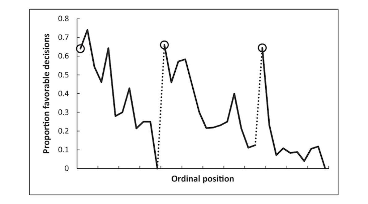
6.3 The Hungry Judges study
In Figure 6.1 we see a graphical representation of the proportion of favorable parole decisions that real-life judges are making as a function of the number of cases they process across the day in Figure 6.1. The study from which this plot is taken is mentioned in many popular science books as an example of a finding that shows that people do not always make rational decisions, but that “judicial rulings can be swayed by extraneous variables that should have no bearing on legal decisions” (Danziger et al., 2011). We see that early on in the day, judges start by giving about 65% of people parole, which basically means, “All right, you can go back into society.” But then very quickly, the number of favorable decisions decreases to basically zero. After a quick break which, as the authors say, “may replenish mental resources by providing rest, improving mood, or by increasing glucose levels in the body” the parole decisions are back up at 65%, and then again quickly drop down to basically zero. They take another break, and the percentage of positive decisions goes back up to 65%, only to drop again over the course of the day.
If we calculate the effect size for the drop after a break, and before the next break (Glöckner, 2016), the effect represents a Cohen’s d of approximately 2, which is incredibly large. There are hardly any effects in psychology this large, let alone effects of mood or rest on decision making. And this surprisingly large effect occurs not just once, but three times over the course of the day. If mental depletion actually has such a huge real-life impact, society would basically fall into complete chaos just before lunch break every day. Or at the very least, our society would have organized itself around this incredibly strong effect of mental depletion. Just like manufacturers take size differences between men and women into account when producing items such as golf clubs or watches, we would stop teaching in the time before lunch, doctors would not schedule surgery, and driving before lunch would be illegal. If a psychological effect is this big, we don’t need to discover it and publish it in a scientific journal - you would already know it exists.
We can look at a meta-meta-analysis (a paper that meta-analyzes a large number of meta-analyses in the literature) by Richard, Bond, & Stokes-Zoota (2003) to see which effect sizes in law psychology are close to a Cohen’s d of 2. They report two meta-analyzed effects that are slightly smaller. The first is the effect that a jury’s final verdict is likely to be the verdict a majority initially favored, which 13 studies show has an effect size of r = .63, or d = 1.62. The second is that when a jury is initially split on a verdict, its final verdict is likely to be lenient, which 13 studies show to have an effect size of r = .63 as well. In their entire database, some effect sizes that come close to d = 2 are the finding that personality traits are stable over time (r = .66, d = 1.76), people who deviate from a group are rejected from that group (r = .6, d = 1.5), or that leaders have charisma (r = .62, d = 1.58). You might notice the almost tautological nature of these effects. And that is, supposedly, the effect size that the passing of time (and subsequently eating lunch) has on parole hearing sentencings.
We see how examining the size of an effect can lead us to identify findings that cannot be caused by their proposed mechanisms. The effect reported in the hungry judges study must therefore be due to a confound. Indeed, such confounds have been identified, as it turns out the ordering of the cases is not random, and it is likely the cases that deserve parole are handled first, and the cases that do not deserve parole are handled later (Chatziathanasiou, 2022; Weinshall-Margel & Shapard, 2011). An additional use of effect sizes is to identify effect sizes that are too large to be plausible. Hilgard (2021) proposes to build in ‘maximum positive controls’, experimental conditions that show the largest possible effect in order to quantify the upper limit on plausible effect size measures.
6.4 Standardised Mean Differences
Conceptually, the d family effect sizes are based on a comparison between the difference between the observations, divided by the standard deviation of these observations. This means that a Cohen’s d = 1 means the standardized difference between two groups equals one standard deviation. The size of the effect in the Facebook study above was quantified with Cohen’s d. Cohen’s d (the d is always italicized) is used to describe the standardized mean difference of an effect. This value can be used to compare effects across studies, even when the dependent variables are measured with different scales, for example when one study uses 7-point scales to measure the dependent variable, while the other study uses a 9-point scale. We can even compare effect sizes across completely different measures of the same construct, for example when one study uses a self-report measure, and another study uses a physiological measure. Although we can compare effect sizes across different measurements, this does not mean they are comparable, as we will discuss in more detail in the section on heterogeneity in the chapter on meta-analysis.
Cohen’s d ranges from minus infinity to infinity (although in practice, the mean difference in the positive or negative direction that can be observed will never be infinite), with the value of 0 indicating that there is no effect. Cohen (1988) uses subscripts to distinguish different versions of d, a practice I will follow because it prevents confusion (without any specification, the term ‘Cohen’s d’ denotes the entire family of effect sizes). Cohen refers to the standardized mean difference between two groups of independent observations for the sample as \(d_s\). Before we get into the statistical details, let’s first visualize what a Cohen’s d of 0.001 (as was found in the Facebook study) means. We will use a visualization from http://rpsychologist.com/d3/cohend/, a website made by Kristoffer Magnusson, that allows you to visualize the differences between two measurements (such as the increase in negative words used by the Facebook user when the number of positive words on the timeline was reduced). The visualization actually shows two distributions, one dark blue and one light blue, but they overlap so much that the tiny difference in distributions is not visible (click the settings button to change the slider settings, and set the step size to 0.001 to reproduce the figure below in the online app).
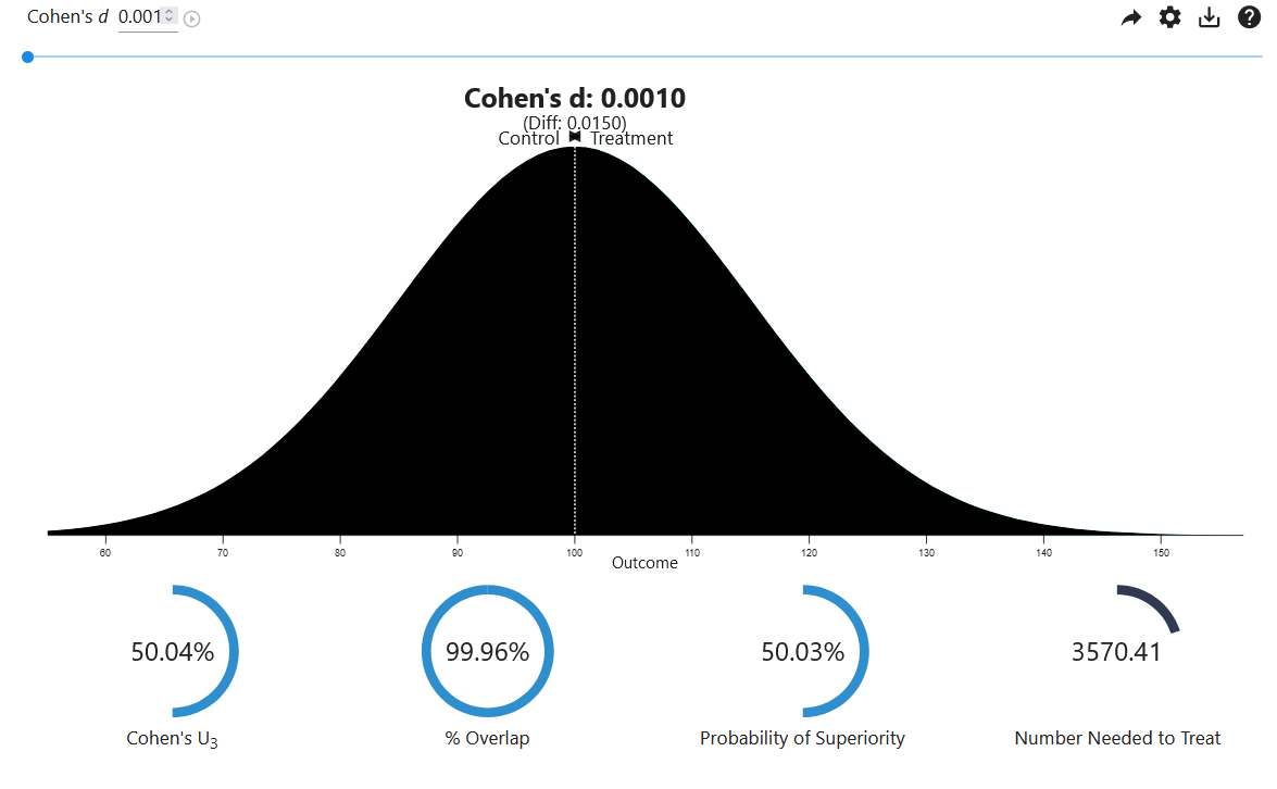
The four numbers below the distribution express the effect size in different ways to facilitate the interpretation. For example, the probability of superiority expresses the probability that a randomly picked observation from one group will have a larger score than a randomly picked observation from the other group. Because the effect is so small, this probability is 50.03% - which means that people in the experimental write almost the same number of positive or negative words as people in the control condition. The number needed to treat index illustrates that in the Facebook study a person needs to type 3,570 words before we will observe one additional negative word, compared to the control condition. This is based on the default setting of the app, where the CER (control event rate, or the number of observations in the control condition that experience an event) is set to 20%. If we set the CER to 2% (rounded from the observed rate of negative words of 1.6%) the number needed to treat becomes 20632. I don’t know how often you type this many words on Facebook, but I think we can agree that this effect is not noticeable on an individual level.
To understand how Cohen’s d for two independent groups is calculated, let’s first look at the formula for the t-statistic:
\[ t = \frac{{\overline{M}}_{1}{- \overline{M}}_{2}}{SD_{pooled} \times \sqrt{\frac{1}{n_{1}} + \frac{1}{n_{2}}}} \]
Here \({\overline{M}}_{1}{- \overline{M}}_{2}\) is the difference between the means, and \(\text{SD}_{\text{pooled}}\) is the pooled standard deviation (Lakens, 2013), and n1 and n2 are the sample sizes of the two groups that are being compared. The t-value is used to determine whether the difference between two groups in a t-test is statistically significant (as explained in the chapter on p-values. The formula for Cohen’s d is very similar:
\[d_s = \frac{{\overline{M}}_{1}{-\overline{M}}_{2}}{SD_{pooled}}\]
As you can see, the sample size in each group (\(n_1\) and \(n_2\)) is part of the formula for a t-value, but it is not part of the formula for Cohen’s d (the pooled standard deviation is computed by weighing the standard deviation in each group by the sample size, but it cancels out if groups are of equal size). This distinction is useful to know, because it tells us that the t-value (and consequently, the p-value) is a function of the sample size, but Cohen’s d is independent of the sample size. If there is a true effect (i.e., a non-zero effect size in the population) the t-value for a null hypothesis test against an effect of zero will on average become larger (and the p-value will become smaller) as the sample size increases. The effect size, however, will not increase or decrease, but will become more accurate, as the standard error decreases as the sample size increases. This is also the reason why p-values cannot be used to make a statement about whether an effect is practically significant, and effect size estimates are often such an important complement to p-values when making statistical inferences.
You can calculate Cohen’s d for independent groups from the independent samples t-value (which can often be convenient when the results section of the paper you are reading does not report effect sizes):
\[d_s = t ⨯ \sqrt{\frac{1}{n_{1}} + \frac{1}{n_{2}}}\]
A d of 0.001 is an extremely tiny effect, so let’s explore an effect size that is a bit more representative of what you would read in the literature. In the meta-meta-analysis mentioned earlier, the median effect size in published studies included in meta-analyses in the psychological literature is d = 0.43 (Richard et al., 2003). To get a feeling for this effect size, let’s use the online app and set the effect size to d = 0.43.
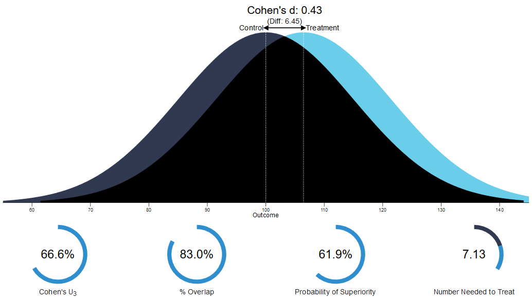
One example of a meta-analytic effect size in the meta-meta-analysis that is exactly \(d_s\) = 0.43 is the finding that people in a group work less hard to achieve a goal than people who work individually, a phenomenon called social loafing. This is an effect that is large enough that we notice it in daily life. Yet, if we look at the overlap in the two distributions, we see that the amount of effort that people put in overlaps considerably between the two conditions (in the case of social loafing, working individually versus working in a group). We see in Figure 6.3 that the probability of superiority, or the probability that if we randomly draw one person from the group condition and one person from the individual condition, the person working in a group puts in less effort, is only 61.9%. This interpretation of differences between groups is also called the common language effect size (McGraw & Wong, 1992).
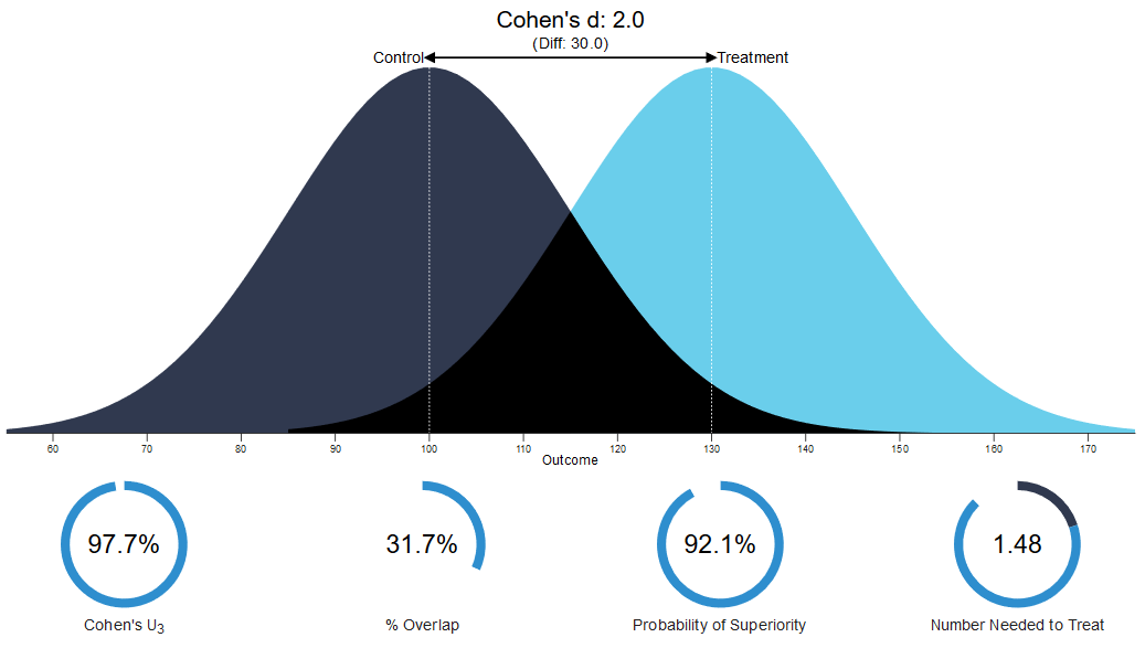
Based on this data, the difference between the height of 21-year old men and women in The Netherlands is approximately 13 centimeters (in an unstandardized effect size), or a standardized effect size of \(d_s\) = 2. If I pick a random man and a random woman walking down the street in my hometown of Rotterdam, how likely is it that the man will be taller than the woman? We see this is quite likely, with a probability of superiority of 92.1%. But even with such a huge effect, there is still considerable overlap in the two distributions. If we conclude that the height of people in one group is greater than the height of people in another group, this does not mean that everyone in one group is taller than everyone in the other group.
Sometimes when you try to explain scientific findings at a birthday party, a skeptical aunt or uncle might remark ‘well I don’t believe that is true because I never experience this’. With probabilistic observations, there is a distribution of observed effects. In the example about social loafing, on average people put in less effort to achieve a goal when working in a group than working by themselves. For any individual in the population, the effect might be larger, smaller, absent, or even in the opposite direction. If your skeptical aunt or uncle never experiences a particular phenomenon, this does not contradict the claim that the effect exists on average in the population. Indeed, it is even expected that there will be no effect for some people in the population, at least some of the time. Although there might be some exceptions (e.g., almost every individual will experience the Stroop effect), many effects are smaller, or have sufficient variation, such that the effect is not present for every single individual in the population.
Conceptually, calculating Cohen’s d for within-subjects comparisons is based on the same idea as for independent groups, where the differences between two observations are divided by the standard deviation within the groups of observations. However, in the case of correlated samples the most common standardizer is the standard deviation of the difference scores. Testing whether two correlated means are significantly different from each other with a paired samples t-test is the same as testing whether the difference scores of the correlated means is significantly different from 0 in a one-sample t-test. Similarly, calculating the effect size for the difference between two correlated means is similar to the effect size that is calculated for a one sample t-test. The standardized mean difference effect size for within-subjects designs is referred to as Cohen’s \(d_z\), where the z alludes to the fact that the unit of analysis is no longer x or y, but their difference, z, and can be calculated with:
\[d_z = \frac{M_{dif}}{\sqrt{\frac{\sum{({X_{dif}-M_{dif})}}^2}{N-1}}}\] The effect size estimate Cohen’s \(d_z\) can also be calculated directly from the t-value and the number of participants using the formula:
\[d_z = \frac{t}{\sqrt{n}}\]
Given the direct relationship between the t-value of a paired-samples t-test and Cohen’s \(d_z\), it is not surprising that software that performs power analyses for within-subjects designs (e.g., G*Power) relies on Cohen’s \(d_z\) as input.
Maxwell & Delaney (2004) remark: ‘a major goal of developing effect size measures is to provide a standard metric that meta-analysts and others can interpret across studies that vary in their dependent variables as well as types of designs.’ Because Cohen’s \(d_z\) takes the correlation between the dependent measures into account, it cannot be directly compared with Cohen’s \(d_s\). Some researchers prefer to use the average standard deviation of both groups of observations as a standardizer (which ignores the correlation between the observations), because this allows for a more direct comparison with Cohen’s \(d_s\). This effect size is referred to as Cohen’s \(d_{av}\) (Cumming, 2013), and is simply:
\[d_{av} = \frac{M_{dif}}{\frac{SD_1+SD_2}{2}}\]
6.5 Interpreting effect sizes
A commonly used interpretation of Cohen’s d is to refer to effect sizes as small (d = 0.2), medium (d = 0.5), and large (d = 0.8) based on benchmarks suggested by Cohen (1988). However, these values are arbitrary and should not be used. In practice, you will only see them used in a form of circular reasoning: The effect is small, because it is d = 0.2, and d = 0.2 is small. We see that using the benchmarks adds nothing, beyond covering up the fact that we did not actually interpret the size of the effect. Furthermore, benchmarks for what is a ‘medium’ and ‘large’ effect do not even correspond between Cohen’s d and r (as explained by McGrath & Meyer (2006); see the ‘Test Yourself’ Q12). Any verbal classification based on benchmarks ignores the fact that any effect can be practically meaningful, such as an intervention that leads to a reliable reduction in suicide rates with an effect size of d = 0.1. In other cases, an effect size of d = 0.1 might have no consequence at all, for example because such an effect is smaller than the just noticeable difference, and is therefore too small to be noticed by individuals in the real world.
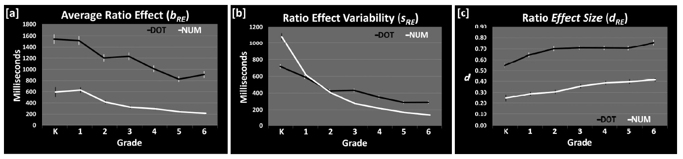
Psychologists rely primarily on standardized effect sizes, where difference scores are divided by the standard deviation. Standardized effect sizes are convenient to compared effects across studies with different measures, and to combine effects in meta-analyses Lakens (2013). However, standardized effect metrics hinder the meaningful interpretation of effects in psychology, as they can reflect either a difference in means, or a difference in standard deviation, or any combination of the two. As an illustrative example, the ratio effect reveals that people find it easier to indicate which of two number represents the larger quantity when the ratio between the numbers is large (e.g., 2 vs. 8) than small (e.g., 4 vs. 5). These numerical comparisons tasks have been used to study the development of numerical processing in children. As noted by Lyons and colleagues (2015), and illustrated in Figure 6.5, the average effect in raw scores (reaction times in milliseconds) declines over grades (pane a). But because the variability declines even more (pane b), the standardized effect size shows the opposite pattern than the raw effect size (pane c). Not surprisingly given this conflicting pattern, the authors ask: “Hence the real question: what is a meaningful effect-size?” (Lyons et al., 2015, p. 1032).
Publication bias and flexibility in the data analysis inflate effect size estimates. Innovations such as Registered Reports (Chambers & Tzavella, 2022; Nosek & Lakens, 2014) increasingly lead to the availability of unbiased effect size estimates in the scientific literature. Registered Reports are scientific publications which have been reviewed before the data has been collected based on the introduction, method, and proposed statistical analysis plan, and published regardless of whether the results were statistically significant or not. One consequence of no longer selectively publishing significant studies is that many effect sizes will turn out to be smaller than researchers thought. For example, in the 100 replication studies performed in the Reproducibility Project: Psychology, observed effect sizes in replication studies were on average half the size of those observed in the original studies (Open Science Collaboration, 2015).
To not just report but interpret an effect size, nothing is gained by the common practice of finding the corresponding verbal label of ‘small’, ‘medium’, or ‘large’. Instead, researchers who want to argue that an effect is meaningful need to provide empirical and falsifiable arguments for such a claim (Anvari et al., 2021; Primbs et al., 2022). One approach to argue that effect sizes are meaningful is by explicitly specifying a smallest effect size of interest, for example based on a cost-benefit analysis. Alternatively, researchers can interpret effect sizes relative to other effects in the literature (Baguley, 2009; Funder & Ozer, 2019).
6.6 Correlations and Variance Explained
The r family effect sizes are based on the proportion of variance that is explained by group membership (e.g., a correlation of r = 0.5 indicates 25% of the variance (\(r^2\)) is explained by the difference between groups). You might remember that r is used to refer to a correlation. The correlation of two continuous variables can range from 0 (completely unrelated) to 1 (perfect positive relationship) or -1 (perfect negative relationship). To get a better feel of correlations, play the interactive game below where you guess the correlation between two variables based on a scatterplot. The game will compute your accuracy across the guesses.
The r family effect sizes are calculated from the sum of squares (the difference between individual observations and the mean for the group, squared and summed) for the effect, divided by the sums of squares for other factors in the design. Earlier, I mentioned that the median effect size in psychology is \(d_s\) = 0.43. However, the authors actually report their results as a correlation, r = 0.21. We can convert Cohen’s d into r (but take care that this only applies to \(d_s\), not \(d_z\)):
\[r = \frac{d_s}{\sqrt{{d_s^{2}}^{+}\frac{N^{2} - 2N}{n_{1} \times n_{2}}}}\]
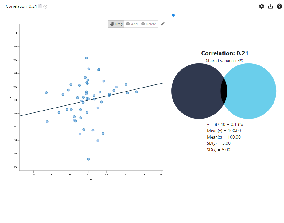
N is the total sample size of both groups, whereas \(n_1\) and \(n_2\) are the sample sizes of the individual groups you are comparing (it is common to use capital \(N\) for the total sample size, and lowercase n for sample sizes per group). You can go to http://rpsychologist.com/d3/correlation/ to look at a good visualization of the proportion of variance that is explained by group membership, and the relationship between r and \(r^2\). The amount of variance explained is often quite a small number, and we see in Figure 6.6 that a correlation of 0.21 (the median from the meta-meta-analysis by Richard and colleagues) we see the proportion of variance explained is only 4.4%. Funder and Ozer (2019) warn against misinterpreting small values for the variance explained as an indication that the effect is not meaningful (and they even consider the practice of squaring the correlation to be “actively misleading”).
As we have seen before, it can be useful to interpret effect sizes to identify effects that are practically insignificant, or those that are implausibly large. Let’s take a look at a study that examines the number of suicides as a function of the amount of country music played on the radio. You can find the paper here. It won an Ig Nobel prize for studies that first make you laugh, and then think, although in this case, the the study should not make you think about country music, but about the importance of interpreting effect sizes.
The authors predicted the following:
We contend that the themes found in country music foster a suicidal mood among people already at risk of suicide and that it is thereby associated with a high suicide rate.
Then they collected data:
Our sample is comprised of 49 large metropolitan areas for which data on music were available. Exposure to country music is measured as the proportion of radio airtime devoted to country music. Suicide data were extracted from the annual Mortality Tapes, obtained from the Inter-University Consortium for Political and Social Research (ICPSR) at the University of Michigan. The dependent variable is the number of suicides per 100,000 population.
And they concluded:
A significant zero-order correlation was found between white suicide rates and country music (r = .54, p < .05). The greater the airtime given to country music, the greater the white suicide rate.
We can again compare the size of this effect with other known effects in psychology. In the database by Richard and colleagues, there are very few effects this large, but some examples are: that leaders are most effective if they have charisma (r = 0.54), good leader–subordinate relations promote subordinate satisfaction (r = 0.53), and people can recognize emotions across cultures (r = 0.53). These effects are all large and obvious, which should raise some doubts about whether the relationship between listening to country music and suicides can be of the same size. Is country music really that bad? If we search the literature, we find that other researchers were not able to reproduce the analysis of the original authors. It is possible that the results are either spurious, or a Type 1 error.
Eta squared, written \(\eta^2\) (part of the r family of effect sizes, and an extension of r that can be used for more than two sets of observations) measures the proportion of the variation in Y that is associated with membership of the different groups defined by X, or the sum of squares of the effect divided by the total sum of squares:
\[\eta^{2} = \frac{\text{SS}_{\text{effect}}}{\text{SS}_{\text{total}}}\]
An \(\eta^2\) of .13 means that 13% of the total variance can be accounted for by group membership. Although \(\eta^2\) is an efficient way to compare the sizes of effects within a study (given that every effect is interpreted in relation to the total variance, all \(\eta^2\) from a single study sum to 100%), eta squared cannot easily be compared between studies, because the total variability in a study (\(SS_{total}\)) depends on the design of a study, and increases when additional variables are manipulated (e.g., when independent variables are added). Keppel (1991) has recommended partial eta squared (\(\eta_{p}^{2}\)) to improve the comparability of effect sizes between studies. \(\eta_{p}^{2}\) expresses the sum of squares of the effect in relation to the sum of squares of the effect plus the sum of squares of the error associated with the effect. Partial eta squared is calculated as:
\[\eta_{p}^{2} = \frac{\text{SS}_{\text{effect}}}{\text{SS}_{\text{effect}} + \text{SS}_{\text{error}}}\]
For designs with fixed factors (manipulated factors, or factors that exhaust all levels of the independent variable, such as alive vs. dead), but not for designs with measured factors or covariates, partial eta squared can be computed from the F-value and its degrees of freedom (Cohen, 1988):
\[\eta_{p}^{2} = \frac{F \times \text{df}_{\text{effect}}}{{F \times \text{df}}_{\text{effect}} + \text{df}_{\text{error}}}\]
For example, for an F(1, 38) = 7.21, \(\eta_{p}^{2}\) = 7.21 /(7.21 ⨯ 1 + 38) = 0.16.
Eta squared can be transformed into Cohen’s d:
d = 2\(\times f\) where \(f^{2} = \eta^{2}/(1 - \eta^{2})\)
6.7 Correcting for Bias
Population effect sizes are almost always estimated on the basis of samples, and as a measure of the population effect size estimate based on sample averages, Cohen’s d slightly overestimates the true population effect. When Cohen’s d refers to the population, the Greek letter \(\delta\) is typically used. Therefore, corrections for bias are used (even though these corrections do not always lead to a completely unbiased effect size estimate). In the d family of effect sizes, the correction for bias in the population effect size estimate of Cohen’s d is known as Hedges’ g (although different people use different names – \(d_{unbiased}\) is also used). This correction for bias is only noticeable in small sample sizes, but since we often use software to calculate effect sizes anyway, it makes sense to always report Hedges’ g instead of Cohen’s d (Thompson, 2007).
As with Cohen’s d, \(\eta^2\) is a biased estimate of the true effect size in the population. Two less biased effect size estimates have been proposed, namely epsilon squared \(\varepsilon^{2}\) and omega squared \(\omega^{2}\). For all practical purposes, these two effect sizes correct for bias equally well (Albers & Lakens, 2018; Okada, 2013), and should be preferred above \(\eta^2\). Partial epsilon squared (\(\varepsilon_{p}^{2}\)) and partial omega squared (\(\omega_{p}^{2}\)) can be calculated based on the F-value and degrees of freedom.
\[ \omega_{p}^{2} = \frac{F - 1}{F + \ \frac{\text{df}_{\text{error}} + 1}{\text{df}_{\text{effect}}}} \]
\[ \varepsilon_{p}^{2} = \frac{F - 1}{F + \ \frac{\text{df}_{\text{error}}}{\text{df}_{\text{effect}}}} \] The partial effect sizes \(\eta_{p}^{2}\), \(\varepsilon_{p}^{2}\) and \(\omega_{p}^{2}\) cannot be generalized across different designs. For this reason, generalized eta-squared (\(\eta_{G}^{2}\)) and generalized omega-squared (\(\omega_{G}^{2}\)) have been proposed (Olejnik & Algina, 2003), although they are not very popular. In part, this might be because summarizing the effect size in an ANOVA design with a single index has limitations, and perhaps it makes more sense to describe the pattern of results, as we will see in the section below.
6.8 Effect Sizes for Interactions
The effect size used for power analyses for ANOVA designs is Cohen’s f. For two independent groups, Cohen’s \(f\) = 0.5 * Cohen’s d. For more than two groups, Cohen’s f can be converted into eta-squared and back with \(f = \frac{\eta^2}{(1 - \eta^2)}\) or \(\eta^2 = \frac{f^2}{(1 + f^2)}\). When predicting interaction effects in ANOVA designs, planning the study based on an expected effect size such as \(\eta_{p}^{2}\) or Cohen’s f might not be the most intuitive approach.
Let’s start with the effect size for a simple two group comparison, and assume we have observed a mean difference of 1, and a standard deviation of 2. This means that the standardized effect size is d = 0.5. An independent t-test is mathematically identical to an F-test with two groups. For an F-test, the effect size used for power analyses is Cohen’s f, which is calculated based on the standard deviation of the population means divided by the population standard deviation (which we know for our measure is 2), or:
\[\begin{equation} f = \frac{\sigma _{ m }}{\sigma} \end{equation}\] where for equal sample sizes \[\begin{equation} \sigma _{ m } = \sqrt { \frac { \sum_ { i = 1 } ^ { k } ( m _ { i } - m ) ^ { 2 } } { k } }. \end{equation}\]
In this formula m is the grand mean, k is the number of means, and \(m_i\) is the mean in each group. The formula above might look a bit daunting, but calculating Cohen’s f is not that difficult for two groups.
If we take the means of 0 and 1, and a standard deviation of 2, the grand mean (the m in the formula above) is (0 + 1)/2 = 0.5. The formula says we should subtract this grand mean from the mean of each group, square this value, and sum them. So we have (0 - 0.5)^2 and (1 - 0.5)^2, which are both 0.25. We sum these values (0.25 + 0.25 = 0.5), divide them by the number of groups (0.5/2 = 0.25), and take the square root, we find that \(\sigma_{ m }\) = 0.5. We can now calculate Cohen’s f (using \(\sigma\) = 2 for our measure):
\[\begin{equation} f = \frac{\sigma _{ m }}{\sigma} = \frac{0.5}{2} = 0.25 \end{equation}\]
We confirm that for two groups Cohen’s f is half as large as Cohen’s d.
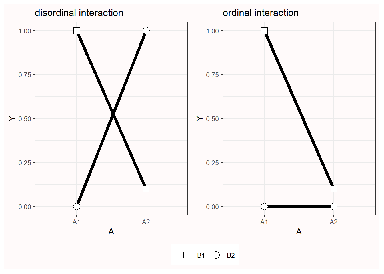
Now we have the basis to look at interaction effects. Different patterns of means in an ANOVA can have the same Cohen’s f. There are two types of interactions, as visualized below in Figure 6.7. In an ordinal interaction, the mean of one group (“B1”) is always higher than the mean for the other group (“B2”). Disordinal interactions are also known as ‘cross-over’ interactions, and occur when the group with the larger mean changes between conditions. The difference is important, since the disordinal interaction in Figure 6.7 has a larger effect size than the ordinal interaction.
Mathematically the interaction effect is computed as the cell mean minus the sum of the grand mean, the marginal mean in each condition of one factor minus the grand mean, and the marginal mean in each condition for the other factor minus grand mean (Maxwell & Delaney, 2004).
Let’s consider two cases, one where we have a perfect disordinal interaction (the means of 0 and 1 flip around in the other condition, and are 1 and 0) or an ordinal interaction (the effect is present in one condition, with means 0 and 1, but disappears in the other condition, with means 0 and 0; see Figure 6.8).
We can calculate the interaction effect as follows (we will go through the steps in some detail). First, let’s look at the disordinal interaction. The grand mean is (1 + 0 + 0 + 1) / 4 = 0.5.
We can compute the marginal means for A1, A2, B1, and B2, which is simply averaging per row and column, which gets us for the A1 row (1+0)/2=0.5. For this perfect disordinal interaction, all marginal means are 0.5. This means there are no main effects. There is no main effect of factor A (because the marginal means for A1 and A2 are both exactly 0.5), nor is there a main effect of B.
We can also calculate the interaction effect. For each cell we take the value in the cell (e.g., for a1b1 this is 1) and compute the difference between the cell mean and the additive effect of the two factors as:
1 - (the grand mean of 0.5 + (the marginal mean of a1 minus the grand mean, or 0.5 - 0.5 = 0) + (the marginal mean of b1 minus the grand mean, or 0.5 - 0.5 = 0)). Thus, for each cell we get:
a1b1: 1 - (0.5 + (0.5 - 0.5) + (0.5 - 0.5)) = 0.5
a1b2: 0 - (0.5 + (0.5 - 0.5) + (0.5 - 0.5)) = -0.5
a2b1: 0 - (0.5 + (0.5 - 0.5) + (0.5 - 0.5)) = -0.5
a2b2: 1 - (0.5 + (0.5 - 0.5) + (0.5 - 0.5)) = 0.5
Cohen’s \(f\) is then \(f = \frac { \sqrt { \frac { 0.5^2 +(-0.5^2) + (-0.5^2) + 0.5^2 } { 4 } }}{ 2 } = 0.25\)
For the ordinal interaction the grand mean is (1 + 0 + 0 + 0) / 4, or 0.25. The marginal means are a1: 0.5, a2: 0, b1: 0.5, and b2: 0.
Completing the calculation for all four cells for the ordinal interaction gives:
a1b1: 1 - (0.25 + (0.5 - 0.25) + (0.5 - 0.25)) = 0.25
a1b2: 0 - (0.25 + (0.5 - 0.25) + (0.0 - 0.25)) = -0.25
a2b1: 0 - (0.25 + (0.0 - 0.25) + (0.5 - 0.25)) = -0.25
a2b2: 0 - (0.25 + (0.0 - 0.25) + (0.0 - 0.25)) = 0.25
Cohen’s \(f\) is then \(f = \frac { \sqrt { \frac { 0.25^2 +(-0.25^2) + (-0.25^2) + 0.25^2 } { 4 } }}{ 2 } = 0.125\).
We see the effect size of the cross-over interaction (f = 0.25) is twice as large as the effect size of the ordinal interaction (f = 0.125). This should make sense if we think about the interaction as a test of contrasts. In the disordinal interaction we are comparing cells a1b1 and a2b2 against a1b2 and a2b1, or (1+1)/2 vs. (0+0)/2. Thus, if we see this as a t-test for a contrast, we see the mean difference is 1. For the ordinal interaction, we have (1+0)/2 vs. (0+0)/2, so the mean difference is halved, namely 0.5. This obviously matters for the statistical power we will have when we examine interaction effects in our experiments.
Just stating that you expect a ‘medium’ Cohen’s f effect size for an interaction effect in your power analysis is not the best approach. Instead, start by thinking about the pattern of means and standard deviations (and for within factors, the correlation between dependent variables) and then compute the effect size from the data pattern. If you prefer not to do so by hand, you can use Superpower (Lakens & Caldwell, 2021). This also holds for more complex designs, such as multilevel models. In these cases, it is often the case that power analyses are easier to perform with simulation-based approaches, than based on plugging a single effect size in to power analysis software (DeBruine & Barr, 2021).
6.9 Why Effect Sizes Selected for Significance are Inflated
Another way to think about this is through the concept of a truncated distribution. If effect sizes are only reported if the p-value is statistically significant, then we only have access to effect sizes that are larger than some minimal value (Anderson et al., 2017; Taylor & Muller, 1996). In the calculator above only effects larger than d = 0.4 can be significant, so all effect sizes below this threshold are censored, and only effect sizes in the gray part of the distribution will be available to researchers. Without the lower part of the effect size distribution effect sizes will on average be inflated.
Estimates based on samples from the population will show variability. The larger the sample, the closer our estimates will be to the true population values, as explained in the next chapter on confidence intervals. Sometimes we will observe larger estimates than the population value, and sometimes we will observe smaller values. As long as we have an unbiased collection of effect size estimates, combining effect sizes estimates through a meta-analysis can increase the accuracy of the estimate. Regrettably, the scientific literature is often biased. It is specifically common that statistically significant studies are published (e.g., studies with p values smaller than 0.05) while studies with p values larger than 0.05 remain unpublished (Franco et al., 2014; Sterling, 1959). Instead of having access to all effect sizes, anyone reading the literature only has access to effects that passed a significance filter. This will introduce systematic bias in our effect size estimates.
To explain how selection for significance introduces bias, it is useful to understand the concept of a truncated or censored distribution. If we want to measure the average length of people in The Netherlands we would collect a representative sample of individuals, measure how tall they are, and compute the average score. If we collect sufficient data the estimate will be close to the true value in the population. However, if we collect data from participants who are on a theme park ride where people need to be at least 150 centimeters tall to enter, the mean we compute is based on a truncated distribution where only individuals taller than 150 cm are included. Smaller individuals are missing. Imagine we have measured the height of two individuals in the theme park ride, and they are 164 and 184 cm tall. Their average height is (164+184)/2 = 174 cm. Outside the entrance of the theme park ride is one individual who is 144 cm tall. Had we measured this individual as well, our estimate of the average length would be (144+164+184)/3 = 164 cm. Removing low values from a distribution will lead to overestimation of the true value. Removing high values would lead to underestimation of the true value.
The scientific literature suffers from publication bias. Non-significant test results – based on whether a p value is smaller than 0.05 or not – are often less likely to be published. When an effect size estimate is 0 the p value is 1. The further removed effect sizes are from 0, the smaller the p value. All else equal (e.g., studies have the same sample size, and measures have the same distribution and variability) if results are selected for statistical significance (e.g., p < .05) they are also selected for larger effect sizes. As small effect sizes will be observed with their corresponding probabilities, their absence will inflate effect size estimates. Every study in the scientific literature provides it’s own estimate of the true effect size, just as every individual provides it’s own estimate of the average height of people in a country. When these estimates are combined – as happens in meta-analyses in the scientific literature – the meta-analytic effect size estimate will be biased (or systematically different from the true population value) whenever the distribution is truncated. To achieve unbiased estimates of population values when combining individual studies in the scientific literature in meta-analyses researchers need access to the complete distribution of values – or all studies that are performed, regardless of whether they yielded a p value above or below 0.05.
In the interactive calculator below we see a distribution centered at an effect size of Cohen’s d = 0.5 for a two-sided t-test with 50 observations in each independent condition. Given an alpha level of 0.05 in this test only effect sizes larger than d = 0.4 will be statistically significant (i.e., all observed effect sizes in the grey area). The threshold for which observed effect sizes will be statistically significant is determined by the sample size and the alpha level (and not influenced by the true effect size). Play around with the values in the calculator to confirm this. The white area under the curve illustrates Type 2 errors – non-significant results that will be observed if the alternative hypothesis is true.
If researchers only have access to the effect sizes estimates in the grey area – a truncated distribution where non-significant results are removed – a weighted average effect size from only these studies will be upwardly biased.
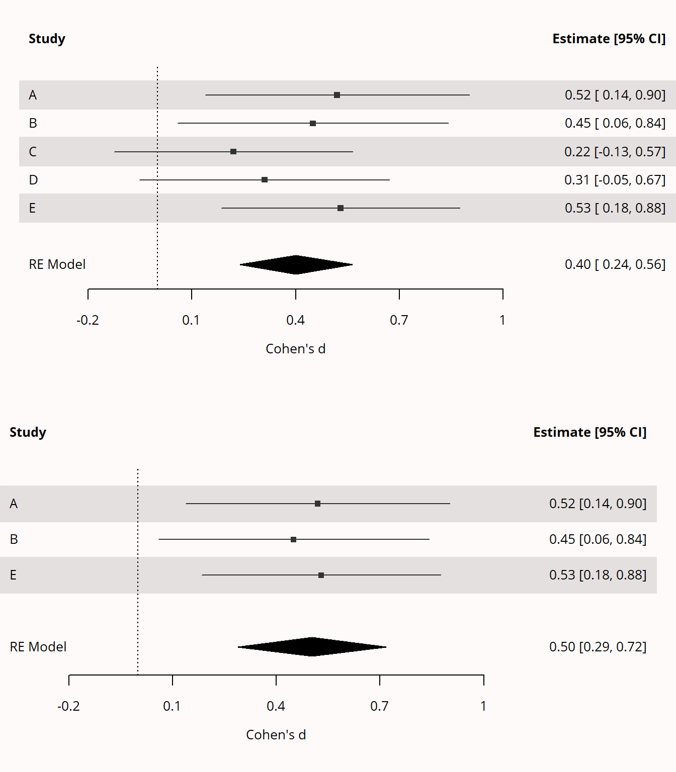
We can see this in the two forest plots visualizing meta-analyses in Figure 6.9. In the top meta-analysis all 5 studies are included, even though study C and D yield non-significant results (as can be seen from the fact that the 95% CI overlaps with 0). The estimated effect size based on all 5 studies is d = 0.4. In the bottom meta-analysis the two non-significant studies are removed - as would happen when there is publication bias. Without these two studies the estimated effect size in the meta-analysis, d = 0.5, is inflated. The extent to which meta-analyses are inflated depends on the true effect size and the sample size of the studies.
The inflation will be greater the larger the part of the distribution is truncated, and the closer the true population effect size is to 0. In our example about the height of individuals the inflation would be greater had we truncated the distribution by removing everyone smaller than 170 cm instead of 150 cm. If the true average height of individuals was 194 cm, removing the few people that are expected to be smaller than 150 (based on the assumption of normally distributed data) would have less of an effect on how much our estimate is inflated than when the true average height was 150 cm, in which case we would remove 50% of individuals. In statistical tests where results are selected for significance at a 5% alpha level more data will be removed if the true effect size is smaller, but also when the sample size is smaller. If the sample size is smaller, statistical power is lower, and more of the values in the distribution (those closest to 0) will be non-significant.
Any single estimate of a population value will vary around the true population value. The effect size estimate from a single study can be smaller than the true effect size, even if studies have been selected for significance. For example, it is possible that the true effect size is 0.5, you have observed an effect size of 0.45, but only effect sizes smaller than 0.4 are truncated when selecting studies based on statistical significance (as in the figure above). At the same time, this single effect size estimate of 0.45 is inflated. What inflates the effect size is the long-run procedure used to generate the value. In the long run effect sizes estimates based on a procedure where estimates are selected for significance will be upwardly biased. This means that a single observed effect size of d = 0.45 will be inflated if it is generated based on a procedure where all non-significant effects are truncated, but it will be unbiased if it is generated based on a distribution where all observed effect sizes are reported, regardless of whether they are significant or not. This also means that a single researcher can not guarantee that the effect sizes they contribute to a literature will contribute to an unbiased effect sizes estimate: There needs to be a system in place where all researchers report all observed effect sizes to prevent bias. An alternative is to not have to rely on other researchers, and collect sufficient data in a single study to have a highly accurate effect size estimate. Multi-lab replication studies are an example of such an approach, where dozens of researchers collect a large number (up to thousands) of observations.
The most extreme consequence of the inflation of effect size estimates occurs when the true effect size in the population is 0, but due to selection of statistically significant results, only significant effects in the expected direction are published. Note that if all significant results are published (and not only effect sizes in the expected direction) 2.5% of Type 1 error rates will be in the positive direction, and 2.5% will be in the negative direction, and the average effect size would be actually be 0. Thus, as long as the true effect size is exactly 0, and all Type 1 errors are published, the effect size estimate would be unbiased. In practice, we see scientists often do not simply publish all results, but only statistically significant results in the desired direction. An example of this is the literature on ego-depletion, where hundreds of studies were published, most showing statistically significant effects, but unbiased large scale replication studies revealed effect sizes of 0 (Hagger et al., 2016; Vohs et al., 2021).
What can be done about the problem of biased effect sizes estimates if we mainly have access to the studies that passed a significance filter? Statisticians have developed approaches to adjust biased effect size estimates by taking a truncated distribution into account (Taylor & Muller, 1996). This approach has recently been implemented in R (Anderson et al., 2017). Implementing this approach in practice is difficult, because we never know for sure if an effect size estimate is biased, and if it is biased, how much bias there is. Furthermore, selection based on significance is only one form of bias, whereas researchers who selectively report significant results may engage in additional problematic research practices, such as selectively reporting results, which are not accounted for in the adjustment. Nevertheless, it can be used as a more conservative approach to estimate effect sizes in a biased literature. Other researchers have referred to this problem as a Type M error (Gelman & Carlin, 2014) and have suggested that researchers always report the average inflation factor of effect sizes. I do not believe this approach is useful. The Type M error is not an error, but a bias in estimation, and it is more informative to compute the adjusted estimate based on a truncated distribution as proposed by Taylor and Muller (1996), than to compute the average inflation for a specific study design. If effects are on average inflated by a factor of 1.3 (the Type M error) it does not mean that the observed effect size is inflated by this factor, and the truncated effect sizes estimator by Taylor and Muller will provide researchers with an actual estimate based on their observed effect size. Type M errors might have a function in education, but they are not useful for scientists.
Of course the real solution to bias in effect size estimates due to significance filters that lead to truncated or censored distributions is to stop selectively reporting results. Designing highly informative studies that have high power to both reject the null, as a smallest effect size of interest in an equivalence test, is a good starting point. Publishing research as Registered Reports is even better. Eventually, if we do not solve this problem ourselves, it is likely that we will face external regulatory actions that force us to include all studies that have received ethical review board approval to a public registry, and update the registration with the effect size estimate, as is done for clinical trials.
6.10 The Minimal Statistically Detectable Effect
Given any alpha level and sample size it is possible to directly compute the minimal statistically detectable effect, or the critical effect size, which is the smallest effect size that, if observed, would be statistically significant given a specified alpha level and sample size (Perugini et al., 2025). As explained in the previous section, if researchers selectively have access to only significant results, all effect sizes should be larger than the minimal statistically detectable effect, and the average effect size estimate will be upwardly inflated. For any critical t value (e.g., t = 1.96 for \(\alpha\) = 0.05, for large sample sizes) we can compute a critical mean difference (Phillips et al., 2001), or a critical standardized effect size. For a two-sided independent t test the critical mean difference is:
\[M_{crit} = t_{crit}{\sqrt{\frac{sd_1^2}{n_1} + \frac{sd_2^2}{n_2}}}\]
and the corresponding critical standardized mean difference is:
\[d_{crit} = t_{crit}{\sqrt{\frac{1}{n_1} + \frac{1}{n_2}}}\]
G*Power provides the critical test statistic (such as the critical t value) when performing a power analysis. For example, Figure 6.10 shows that for a correlation based on a two-sided test, with \(\alpha\) = 0.05, and N = 30, only effects larger than r = 0.361 or smaller than r = -0.361 can be statistically significant. This reveals that when the sample size is relatively small, the observed effect needs to be quite substantial to be statistically significant.

It is important to realize that due to random variation each study has a probability to yield effects larger than the critical effect size, even if the true effect size is small (or even when the true effect size is 0, in which case each significant effect is a Type I error). At the same time, researchers often do not want to perform an experiment where effects they are interested in can not even become statistically significant, which is why it can be useful to compute the minimal statistically significant effect as part of a sample size justification.
6.11 Test Yourself
Q1: One of the largest effect sizes in the meta-meta analysis by Richard and colleagues from 2003 is that people are likely to perform an action if they feel positively about the action and believe it is common. Such an effect is (with all due respect to all of the researchers who contributed to this meta-analysis) somewhat trivial. Even so, the correlation was r = .66, which equals a Cohen’s d of 1.76. What, according to the online app at https://rpsychologist.com/cohend/, is the probability of superiority for an effect of this size?
Q2: Cohen’s d is to ______ as eta-squared is to ________
Q3: A correlation of r = 1.2 is:
Q4: Let’s assume the difference between two means we observe is 1, and the pooled standard deviation is also 1. If we simulate a large number of studies with those values, what, on average, happens to the t-value and Cohen’s d, as a function of the sample size in these simulations?
Q5: Go to http://rpsychologist.com/d3/correlation/ to look at a good visualization of the proportion of variance that is explained by group membership, and the relationship between r and \(r^2\). Look at the scatterplot and the shared variance for an effect size of r = .21 (Richard et al., 2003). Given that r = 0.21 was their estimate of the median effect size in psychological research (not corrected for bias), how much variance in the data do variables in psychology on average explain?
Q6: By default, the sample size for the online correlation visualization linked to above is 50. Click on the cogwheel to access the settings, change the sample size to 500, and click the button ‘New Sample’. What happens?
Q7: In an old paper you find a statistical result reported as t(36) = 2.14, p < 0.05 for an independent t-test without a reported effect size. Using the online MOTE app https://doomlab.shinyapps.io/mote/ (choose “Independent t -t” from the Mean Differences dropdown menu) or the MOTE R function d.ind.t.t, what is the Cohen’s d effect size for this effect, given 38 participants (e.g., 19 in each group, leading to N – 2 = 36 degrees of freedom) and an alpha level of 0.05?
Q8: In an old paper you find a statistical result from a 2x3 between-subjects ANOVA reported as F(2, 122) = 4.13, p < 0.05, without a reported effect size. Using the online MOTE app https://doomlab.shinyapps.io/mote/ (choose Eta – F from the Variance Overlap dropdown menu) or the MOTE R function eta.F, what is the effect size expressed as partial eta-squared?
Q9: You realize that computing omega-squared corrects for some of the bias in eta-squared. For the old paper with F(2, 122) = 4.13, p < 0.05, and using the online MOTE app https://doomlab.shinyapps.io/mote/ (choose Omega – F from the Variance Overlap dropdown menu) or the MOTE R function omega.F, what is the effect size in partial omega-squared? HINT: The total sample size is the \(df_{error} + k\), where k is the number of groups (which is 6 for the 2x3 ANOVA).
Q10: Several times in this chapter the effect size Cohen’s d was converted to r, or vice versa. We can use the effectsize R package (that can also be used to compute effect sizes when you analyze your data in R) to convert the median r = 0.21 observed in Richard and colleagues’ meta-meta-analysis to d: effectsize::r_to_d(0.21) which (assuming equal sample sizes per condition) yields d = 0.43 (the conversion assumes equal sample sizes in each group). Which Cohen’s d corresponds to a r = 0.1?
Q11: It can be useful to convert effect sizes to r when performing a meta-analysis where not all effect sizes that are included are based on mean differences. Using the d_to_r() function in the effectsize package, what does a d = 0.8 correspond to (again assuming equal sample sizes per condition)?
Q12: From questions 10 and 11 you might have noticed something peculiar. The benchmarks typically used for ‘small’, ‘medium’, and ‘large’ effects for Cohen’s d are d = 0.2, d = 0.5, and d = 0.8, and for a correlation are r = 0.1, r = 0.3, and r = 0.5. Using the d_to_r() function in the effectsize package, check to see whether the benchmark for a ‘large’ effect size correspond between d and r.
As McGrath & Meyer (2006) write: “Many users of Cohen’s (1988) benchmarks seem unaware that those for the correlation coefficient and d are not strictly equivalent, because Cohen’s generally cited benchmarks for the correlation were intended for the infrequently used biserial correlation rather than for the point biserial.”
Download the paper by McGrath and Meyer, 2006 (you can find links to the pdf here), and on page 390, right column, read which solution the authors prefer.
6.11.1 Open Questions
What is the difference between standardized and unstandardized effect sizes?
Give a definition of an ‘effect size’.
What are some of the main uses of effect sizes?
How can effect sizes improve statistical inferences, beyond looking at the p-value?
What is the effect size r, and which values can it take?
What is the effect size d, and which values can it take?
What are the unbiased effect sizes that correspond to d and eta-squared called?
Give an example when small effects are meaningless, and when they are not.
Researchers often use Cohen’s (1988) benchmarks to interpret effect sizes. Why is this not best practice?
What is the difference between ordinal and disordinal interaction effects? And if the means across different conditions are either 0 or 1 on a scale, which type of interaction will have a larger effect size?