2  Social computing using R

This part will introduce you to R and the `igraph’ package.

Intended Learning Outcomes:

• install R and Rstudio
• define network objects
• inspect network objects
• read network data
• select sub-networks

R is an ideal platform for developing and conducting network analyses. The R statistical programming language and environment comprise a vast integrated system of thousands of packages and functions that allow it to handle innumerable data management, analysis, or visualization tasks.

The R system includes a number of packages that are designed to accomplish specific network analytic tasks.However, by performing these network tasks within the R environment, the analyst can take advantage of any of the other capabilities of R. Most other network analysis programs (e.g., Pajek, UCINet, Gephi) are stand-alone packages, and thus do not have the advantages of working within an integrated statistical programming environment. See for a comparison of various network tools

https://sci2s.ugr.es/sites/default/files/files/Teaching/GraduatesCourses/RedesSistemasCompejos/wias_2010-Comparativa-SNA-tools.pdf

By pairing R up with an integrated development environment (IDE) such as RStudio and taking advantage of packages such as knitr and shiny, the user has the ability to manage any type of complex network project. In fact, the development and availability of these tools has been one of the driving forces of the reproducible research movement, which emphasizes the importance of combining data, code, results, and documentation in permanent and shareable forms.

There are various network analysis packages available in R. Basic network analysis and visualization can be handled with the sna package contained within the much broader statnet suite of network packages. Sophisticated modeling of network dynamics can be handled by ergm and its associated libraries, and dynamic actor-based network models are produced by RSiena.

Being open source, users from around the world add new functions to its repositories on a daily basis. This means that the possible tools you can use and analyses you can perform with R are expanding constantly, making it an increasingly powerful environment for statistical analysis. We will show you just a glimpse of this power, but hopefully we can provide enough of a basis for you to go out on your own and learn more. In the course we will make use of R to visualize networks and perform network analysis.

If you have not already done so, install R and Rstudio. First install R, you can find it on the “Comprehensive R Archive Network:

https://cran.r-project.org/.

Then, install R studio, which makes life so much easier:

https://www.rstudio.com/products/rstudio/download/.

The best way to learn the necessary basics of R is to use the swirl R package, an interactive, easy way to learn R programming in the R environment.

2.1 A tutorial in R: Swirl

I assume that you installed R and RStudio. Open RStudio and type the following into the console.

install.packages("swirl")

Note that the > symbol at the beginning of the line is R’s prompt for you type something into the console. We include it here so you know that this command is to be typed into the console and not elsewhere. The part you type begins after “>”.

Starting swirl is the only step that you will repeat every time you want to run swirl. First, you will load the package using the library() function. Then you will call the function that starts the magic! Type the following, pressing Enter (or Ctrl + Enter on my machine) after each line:

library("swirl")

swirl()

The last step is to install an interactive course, and follow it. The first time you start swirl, you’ll be prompted to install a course. You can either install one of the recommended courses or visit our course repository for more options. There are even more courses available from the Swirl Course Network.

If you’d like to install a course that is not part of our course repository, type

?InstallCourses

at the R prompt for a list of functions that will help you do so. The best course to start if you are an absolute beginner in R is the very short introduction to R by Claudia Brauer. Run the following code in your R console.

swirl::install_course("A_(very)_short_introduction_to_R")

After swirl() you can select the course and its modules. Complete the course, and you will have no trouble following the course SNA in R (at least not with the R part!).

2.2 Defining network objects

A major advantage of using R for network analysis is the power and flexibility of the tools for accessing and manipulating the actual network data. In this section we will learn how to create network data objects. In a next section we discuss how network from existing data sources can be entered into R and turned into a network data object. Finally, a number of typical network data management tasks are illustrated.

Install the latest version of the package “igraph”.

install.packages("igraph")

Note that igraph should be started via library(igraph) while this is always needed in the remainder, I will not display it in the code as to reduce the output.

2.2.1 the graph command

The way that graphs are created, stored and manipulated in R bears a strong resemblance to how they are defined and studied algebraically. A graph \(G\) consists of two sets. The first set \(V\) is known as the vertex set or node set. The second set \(E\) is known as the edge set, and consists of pairs of elements of \(V\). Given that a graph is made up of these two sets, we will often notate our graph as \(G=(V,E)\). If two vertices appear as a pair in \(E\), then those vertices are said to be adjacent or connected vertices.

Let’s use an example to illustrate this definition. The Figure below is a diagram of a graph \(G_{HTI}\) with four vertices representing four professors of our HTI department. An edge connects two vertices if and only if those two people have closely worked together.

G <- graph(edges=c("Uwe","Gerrit","Uwe", "Rianne","Gerrit","Martijn","Rianne","Martijn"), directed= F) 

# A simple plot of the network - we'll talk more about plots later
plot(G, asp=0.6) 

Our vertex set \(V\) for the graph \(G_{HTI}\) is is:

\(V=\{Uwe, Gerrit, Rianne, Martijn\}\).

The edge set is defined as pairs of elements of the vertex set.

\(E=\{\{Uwe, Gerrit\},\{Uwe,Rianne\},\{Gerrit,Martijn\},\{Rianne,Martijn\}\}\)

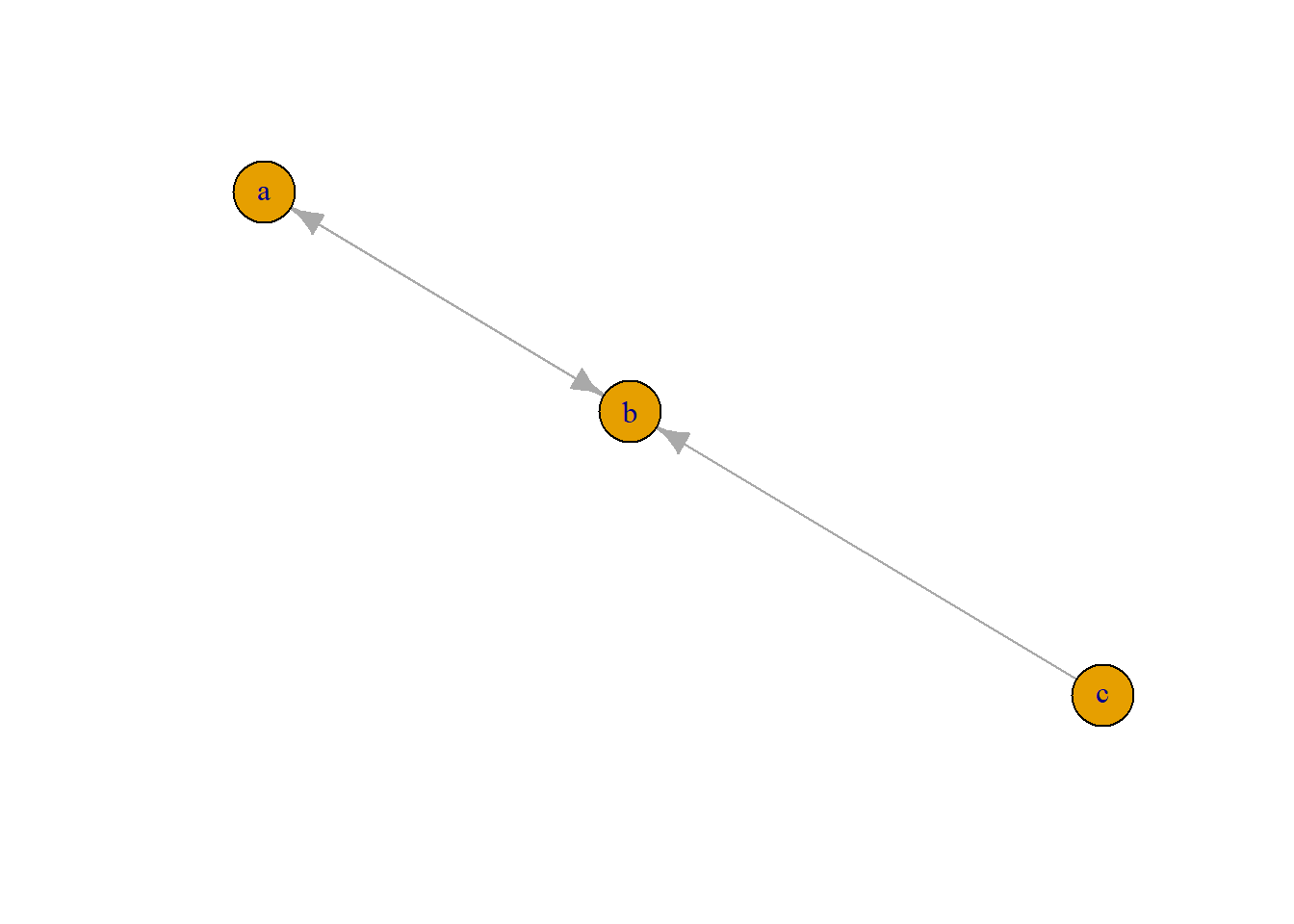
In the graph command above, we specified that the graph is undirected (“directed=F”). This makes sense obviously, since if Uwe works closely with Gerrit, Gerrit works closely with Uwe. If we do not specify that the graph is undirected, igraph by default assumes that edges are directed (indicating for instance a “x likes y” relationship). As can be verified in the Figure the order of the vertices in the pairs matters.

G <- graph(edges=c("Uwe","Gerrit","Uwe", "Rianne","Gerrit","Martijn","Rianne","Martijn")) 
plot(G, asp=0.6) 

There are various ways of creating a network graph in Igraph. The graph command is straightforward. The graph function allows to add isolated vertices. Isolates do not have connections to other vertices, so adding them increases the vertex set, but not the edge set.

g3 <- graph(edges=c("Uwe","Gerrit","Uwe", "Rianne","Gerrit","Martijn","Rianne","Martijn"),isolates=c("Sanne", "Peter"),  directed= F) 
plot(g3, asp=0.6)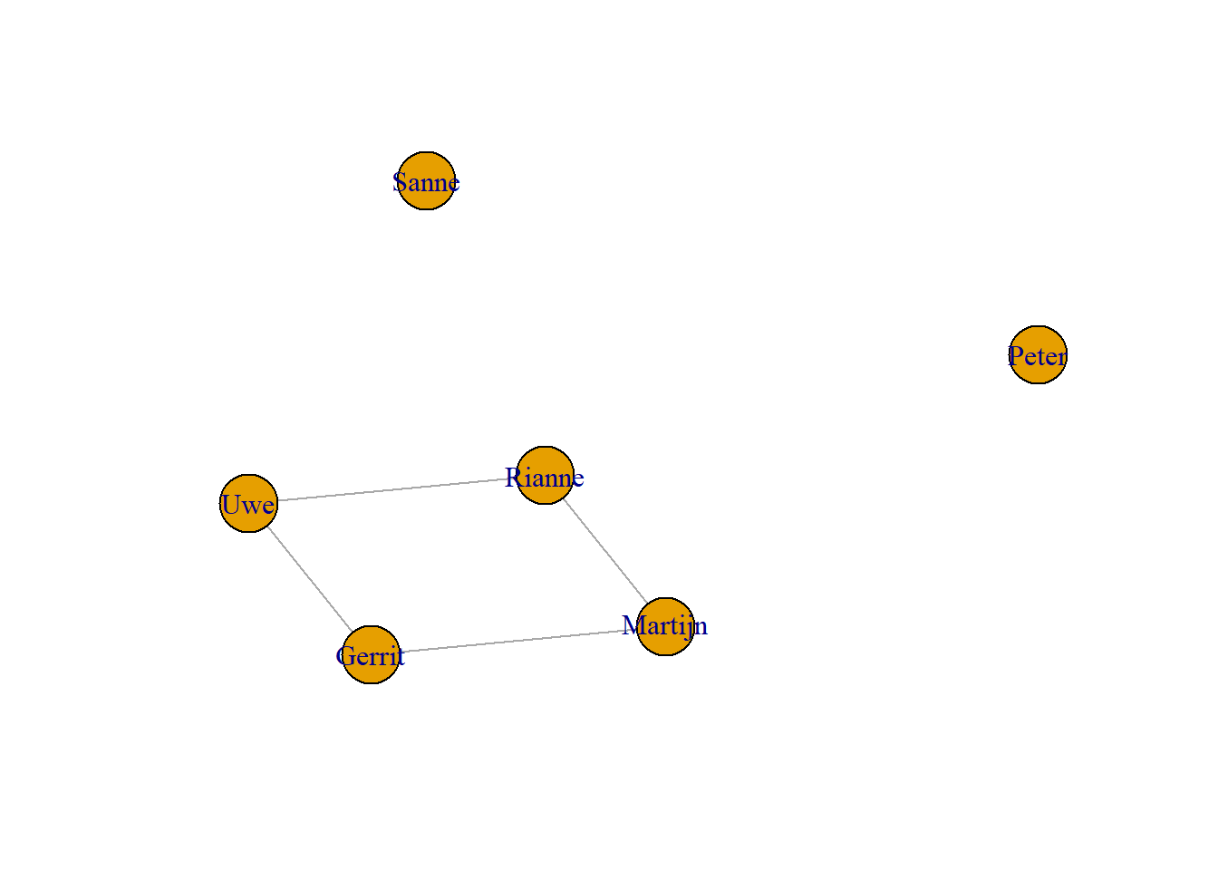

The graph above is a so-called simple graph since there are no multiple relations between vertices. In a multiple graph this is allowed. An example could be a combination of “x manages y” and “x likes y” relations. Multiple graphs are not common in social network analysis (we will not further discuss them in this course).

multi_graph <- graph(edges=c("Uwe","Gerrit","Uwe", "Rianne", "Uwe", "Rianne", "Gerrit","Martijn","Rianne","Martijn")) 
plot(multi_graph, asp=0.6) 

In a pseudo graph vertices are allowed to connect to themselves (self-loops). This can for instance happen in a “x emails y” network relation, since we can send ourselves an email. In practice (and in our course) self-loops (and pseudo graphs) are not of interest in social network analysis.

pseudo_graph <- graph(edges=c("Uwe","Uwe","Uwe","Gerrit","Uwe", "Rianne","Gerrit","Martijn","Rianne","Martijn")) 
plot(pseudo_graph, asp=0.6) 

2.2.2 the graph_from_literal command

An somewhat easier alternative to the graph command is the graph_from_literal command. It uses more intuitive symbols for relations: ‘-’ for undirected tie, “+-’ or”-+” for directed ties pointing left & right, “++” for a symmetric tie, and “:” for sets of vertices

plot(graph_from_literal(a---b, b---c), asp=0.6) 

plot(graph_from_literal(a+-+b, b+--c), asp=0.6)

The ‘:’ operator can be used to define vertex sets. If an edge operator connects two vertex sets then every vertex from the first set will be connected to every vertex in the second set.

plot(graph_from_literal(Alice - Bob:Cecil:Daniel, Cecil:Daniel - Eugene:Gordon))

2.2.3 Adding attributes to a graph

A graph \(G=(V,E)\) consists of a vertex set \(V\) and an edge set \(E\). These sets are the minimum elements of a graph—the vertices represent the entities in the graph and the edges represent the relationships between the entities. We can enhance a graph to provide even richer information on the entities and on the relationships by giving our vertices and edges properties. A vertex property provides more specific information about a vertex and an edge property provides more specific information about the relationship between two vertices.

We could for instance include the gender attribute. We can notate properties as additional sets in our graph, ensuring that each entry is in the same order as the respective vertices or edges, as follows:

\(V=\{Uwe, Gerrit, Rianne, Martijn\}\).

\(V_{gender}=\{male, male, female, male\}\).

Note that the vertex property set \(V_{gender}\) has the same number of elements as \(V\) and the associated properties appear in the same order as the vertices of \(V\)’. Vertex and edge properties can be added to a new graph at the point of creation or can be added progressively to an existing graph. We will first focus on adding them to an existing graph object in igraph.

# First note that the vertex set can be easily accessed. 
V(G)

+ 4/4 vertices, named, from 2c04b06:
[1] Uwe     Gerrit  Rianne  Martijn

#Second the names are stored automatically, and can be accessed as well.
V(G)$name 

[1] "Uwe"     "Gerrit"  "Rianne"  "Martijn"

The $ operator is used to extract or subset a specific part of a data object in R. For instance, this can be a data frame object or a list. We can use this operator to add a vertex attribute to the igraph object.

# note that the c() function creates a vector .
V(G)$gender <- c("male", "male", "female", "male")

The procedure in igraph is similar for edge attributes. Here we include an edge attribute “type of relation”. Again we must make sure that each entry is in the same order as the respective edges:

E(G)

+ 4/4 edges from 2c04b06 (vertex names):
[1] Uwe   ->Gerrit  Uwe   ->Rianne  Gerrit->Martijn Rianne->Martijn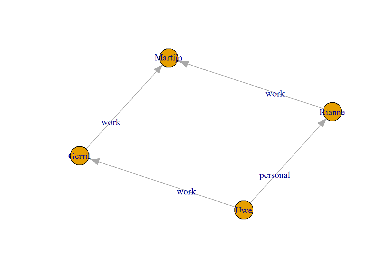

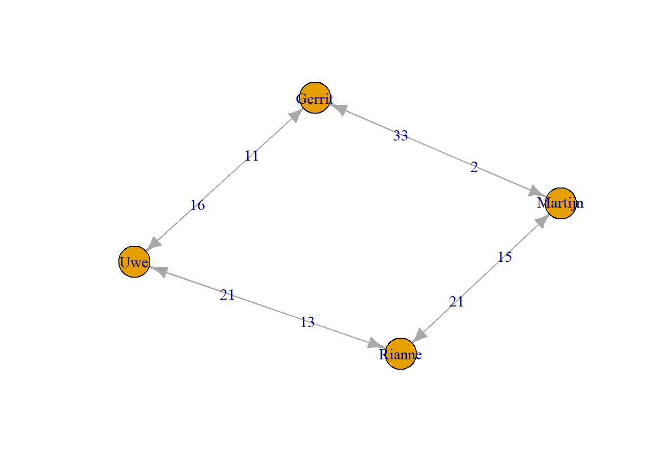
E(G)$type<-c("work","personal", "work", "work")
plot(G, edge.label=E(G)$type, asp=0.6)

In the example above the edges were provided with a categorical label. Edges can have (continuous) weights as well. A well known example are communication networks, where the weight indicates the interaction frequency. Networks where relations have weights are called weighted networks. For instance, suppose that in the \(G\) network we are now interested in how often HTI members send emails to each other (monthly).

G <- graph(edges=c("Uwe","Gerrit", "Gerrit", "Uwe","Uwe", "Rianne", "Rianne", "Uwe", "Gerrit","Martijn", "Martijn", "Gerrit", "Rianne","Martijn","Martijn", "Rianne")) 
E(G)$weight <- c(16, 11,21,13, 33,2,21, 15) 
plot(G, edge.label=E(G)$weight, asp=0.6)

2.3 Examing network data

Whether you import a network (more about that later), or create a network (like above), it is always a good idea to inspect the network and explore whether data entry mistakes or other mistakes were made (just like in normal data analysis practice). When we visually inspect the plot of g3 earlier we can see it has two edges going from Jim to Jack, and a loop from John to himself.

For larger networks this is, not always easy to see. An easy command that answers whether there are multiple links between vertices, or self-loops is the is.simple command.

G <- graph(edges=c("Uwe","Gerrit", "Gerrit", "Gerrit", "Uwe", "Rianne", "Uwe", "Rianne", "Gerrit","Martijn","Rianne","Martijn"), directed= F) 
plot(G, asp=0.6)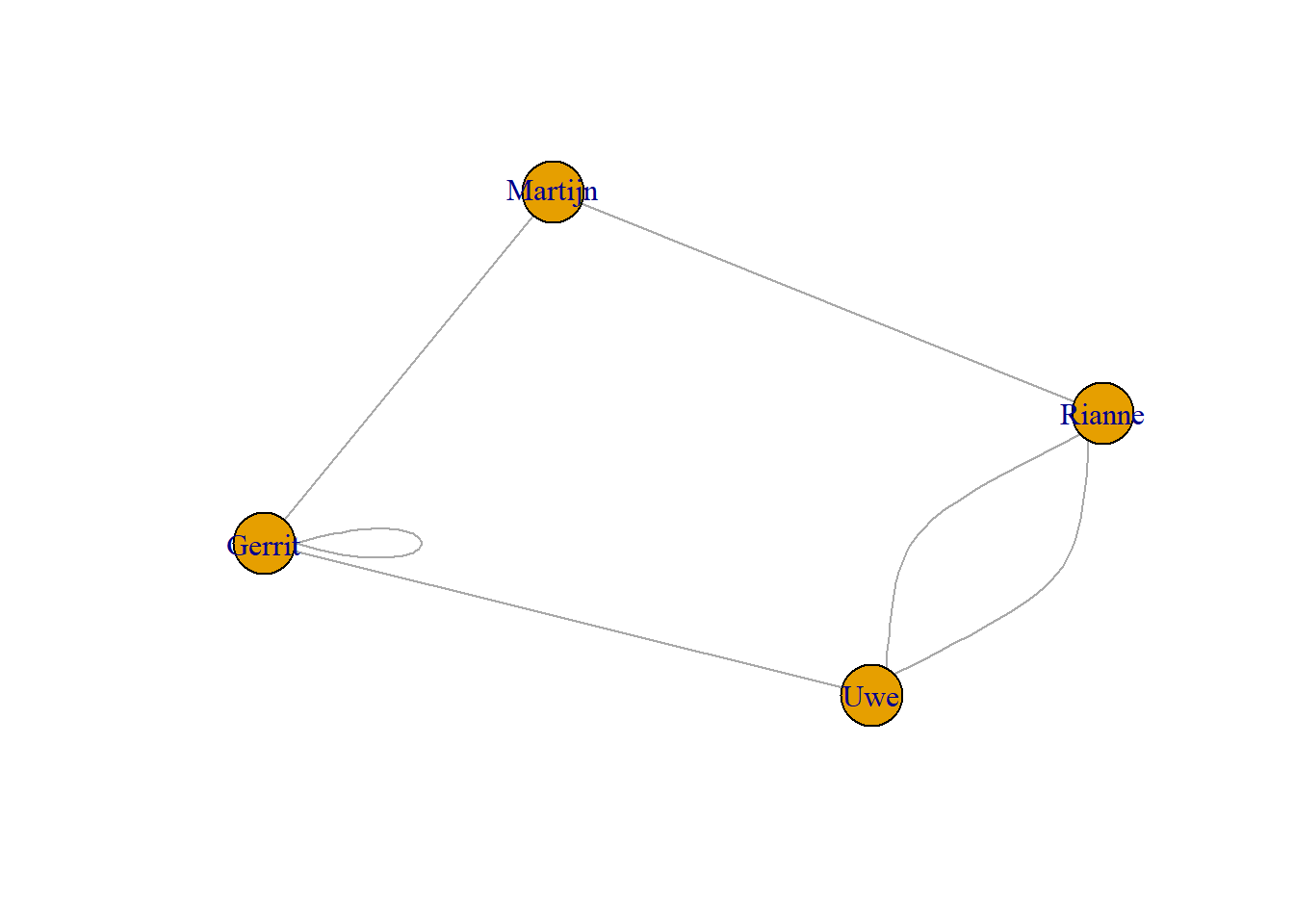

is.simple(G)

[1] FALSE

You may want to know which relations are multiple or self-loops. Relation number two is the self-loop, and relation number five is the multiple relation.

E(G)

+ 6/6 edges from 2d0bc32 (vertex names):
[1] Uwe   --Gerrit  Gerrit--Gerrit  Uwe   --Rianne  Uwe   --Rianne 
[5] Gerrit--Martijn Rianne--Martijn

which_loop(G)

[1] FALSE  TRUE FALSE FALSE FALSE FALSE

which_multiple(G)

[1] FALSE FALSE FALSE  TRUE FALSE FALSE

We can simplify our graph to remove loops & multiple edges between the same nodes using the simplify command (default is that you remove multiple edges and self-loops, but this can be adjusted).

sG<-igraph::simplify(G)
sG[] #inspect the matrix (dots are zeros)

4 x 4 sparse Matrix of class "dgCMatrix"
        Uwe Gerrit Rianne Martijn
Uwe       .      1      1       .
Gerrit    1      .      .       1
Rianne    1      .      .       1
Martijn   .      1      1       .

You can inspect the edges and vertices of a network, and inspect the network as a whole or specific rows, columns, or cells as follows:

sG[1,]

    Uwe  Gerrit  Rianne Martijn 
      0       1       1       0 

sG[1,1]

[1] 0

edge_attr(sG)

named list()

vertex_attr(sG)

$name
[1] "Uwe"     "Gerrit"  "Rianne"  "Martijn"

graph_attr(sG)

named list()

We will discuss three main ways of entering network data: edgelist data, adjance matrices, and two mode network data.

2.4 Reading edge list data

One simple way to represent a graph is to list the edges, which we will refer to as an edge list. For each edge, we just list who that edge is incident on. Edge lists are therefore two column matrices that directly tell the computer which actors are tied for each edge. In a directed graph, the actors in column A are the sources of edges, and the actors in Column B receive the tie. In an undirected graph, order doesn’t matter.

In R, we can create an example edge list using vectors and data.frames. I specify each column of the edge list with vectors and then assign them as the columns of a data.frame. We can use this to visualize what an edge list should look like.

personA <- c("Mark", "Mark", "Peter", "Peter", "Bob", "Jill")
personB <- c("Peter", "Jill", "Bob", "Aaron", "Jill", "Aaron")

edgelist <- data.frame(PersonA = personA, PersonB = personB, stringsAsFactors = F)

print(edgelist)

  PersonA PersonB
1    Mark   Peter
2    Mark    Jill
3   Peter     Bob
4   Peter   Aaron
5     Bob    Jill
6    Jill   Aaron

There are at least two ways to read edge list data. The example that is shown here use the graph_from_data_frame command. A simpler command graph.edgelist can be used if the data only contains two columns (edges from to).

The data set we are using as an example consists of two files, Dataset1-Media-Example- NODES.csv and Dataset1-Media-Example-EDGES.csv

nodes<-read.csv("data/Dataset1-Media-Example-NODES.csv")
links<-read.csv("data/Dataset1-Media-Example-EDGES.csv")

head(nodes)

id	media	media.type	type.label	audience.size
s01	NY Times	1	Newspaper	20
s02	Washington Post	1	Newspaper	25
s03	Wall Street Journal	1	Newspaper	30
s04	USA Today	1	Newspaper	32
s05	LA Times	1	Newspaper	20
s06	New York Post	1	Newspaper	50

head(links)

from	to	weight	type
s01	s02	10	hyperlink
s01	s02	12	hyperlink
s01	s03	22	hyperlink
s01	s04	21	hyperlink
s04	s11	22	mention
s05	s15	21	mention

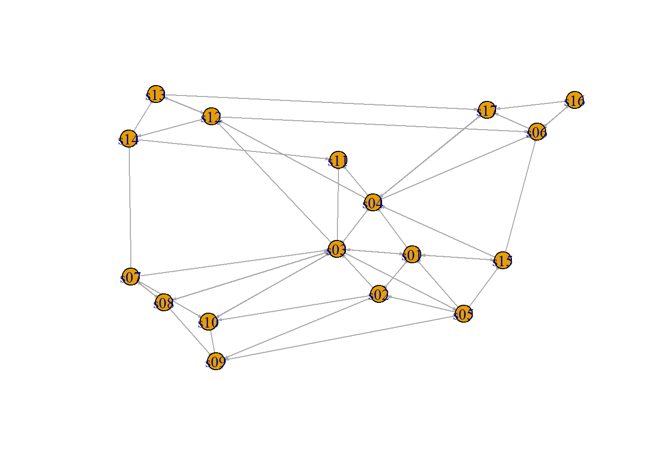
Next we will convert the raw data to an igraph network object. To do that, we will use the graph_from_data_frame() function, which takes two data frames: d and vertices.

• d describes the edges of the network. Its first two columns are the IDs of the source and the target node for each edge. The following columns are edge attributes (weight, type, label, or anything else).

• vertices starts with a column of node IDs. Any following columns are interpreted as node attributes.

net <- graph_from_data_frame(d=links, vertices=nodes, directed=T)
net

IGRAPH 2e966d8 DNW- 17 52 -- 
+ attr: name (v/c), media (v/c), media.type (v/n), type.label (v/c),
| audience.size (v/n), weight (e/n), type (e/c)
+ edges from 2e966d8 (vertex names):
 [1] s01->s02 s01->s02 s01->s03 s01->s04 s04->s11 s05->s15 s06->s17 s08->s09
 [9] s08->s09 s03->s04 s04->s03 s01->s15 s15->s01 s15->s01 s16->s17 s16->s06
[17] s06->s16 s09->s10 s08->s07 s07->s08 s07->s10 s05->s02 s02->s03 s02->s01
[25] s03->s01 s12->s13 s12->s14 s14->s13 s13->s12 s05->s09 s02->s10 s03->s12
[33] s04->s06 s10->s03 s03->s10 s04->s12 s13->s17 s06->s06 s14->s11 s03->s11
[41] s12->s06 s04->s17 s17->s04 s08->s03 s03->s08 s07->s14 s15->s06 s15->s04
[49] s05->s01 s02->s09 s03->s05 s07->s03

Above we already briefly discussed this description. The description of an igraph object starts with four letters:

1. D or U, for a directed or undirected graph

2. N for a named graph (where nodes have a name attribute)

3. W for a weighted graph (where edges have a weight attribute)

4. B for a bipartite (two-mode) graph (where nodes have a type attribute)

The two numbers that follow (17 52) refer to the number of nodes and edges in the graph. The description also lists node & edge attributes, for example:

• (g/c) graph-level character attribute.

• (v/c) vertex-level character attribute. So “name” is a vertex level attribute. The c indicates that this attribute is a character object, which is used to represent string values in R.

• (e/n) edge-level numeric attribute. The “weight” edge attribute refers to how often one media source refers to another (and hence is numerical)

We have easy access to nodes, edges, and their attributes with the following code.

E(net) # The edges of the "net" object

+ 52/52 edges from 2e966d8 (vertex names):
 [1] s01->s02 s01->s02 s01->s03 s01->s04 s04->s11 s05->s15 s06->s17 s08->s09
 [9] s08->s09 s03->s04 s04->s03 s01->s15 s15->s01 s15->s01 s16->s17 s16->s06
[17] s06->s16 s09->s10 s08->s07 s07->s08 s07->s10 s05->s02 s02->s03 s02->s01
[25] s03->s01 s12->s13 s12->s14 s14->s13 s13->s12 s05->s09 s02->s10 s03->s12
[33] s04->s06 s10->s03 s03->s10 s04->s12 s13->s17 s06->s06 s14->s11 s03->s11
[41] s12->s06 s04->s17 s17->s04 s08->s03 s03->s08 s07->s14 s15->s06 s15->s04
[49] s05->s01 s02->s09 s03->s05 s07->s03

V(net) # The vertices of the "net" object

+ 17/17 vertices, named, from 2e966d8:
 [1] s01 s02 s03 s04 s05 s06 s07 s08 s09 s10 s11 s12 s13 s14 s15 s16 s17

E(net)$type # Edge attribute "type"

 [1] "hyperlink" "hyperlink" "hyperlink" "hyperlink" "mention"   "mention"  
 [7] "mention"   "mention"   "mention"   "hyperlink" "hyperlink" "mention"  
[13] "hyperlink" "hyperlink" "mention"   "hyperlink" "hyperlink" "mention"  
[19] "mention"   "mention"   "hyperlink" "hyperlink" "hyperlink" "hyperlink"
[25] "hyperlink" "hyperlink" "mention"   "mention"   "hyperlink" "hyperlink"
[31] "hyperlink" "hyperlink" "mention"   "hyperlink" "mention"   "hyperlink"
[37] "mention"   "hyperlink" "mention"   "hyperlink" "mention"   "mention"  
[43] "hyperlink" "hyperlink" "hyperlink" "mention"   "hyperlink" "hyperlink"
[49] "mention"   "hyperlink" "hyperlink" "mention"  

V(net)$media # Vertex attribute "media"

 [1] "NY Times"            "Washington Post"     "Wall Street Journal"
 [4] "USA Today"           "LA Times"            "New York Post"      
 [7] "CNN"                 "MSNBC"               "FOX News"           
[10] "ABC"                 "BBC"                 "Yahoo News"         
[13] "Google News"         "Reuters.com"         "NYTimes.com"        
[16] "WashingtonPost.com"  "AOL.com"            

You can also find nodes and edges using attribute information. This can be useful when we want to color vertices and edges.

V(net)[media=="BBC"]

+ 1/17 vertex, named, from 2e966d8:
[1] s11

E(net)[type=="mention"]

+ 21/52 edges from 2e966d8 (vertex names):
 [1] s04->s11 s05->s15 s06->s17 s08->s09 s08->s09 s01->s15 s16->s17 s09->s10
 [9] s08->s07 s07->s08 s12->s14 s14->s13 s04->s06 s03->s10 s13->s17 s14->s11
[17] s12->s06 s04->s17 s07->s14 s05->s01 s07->s03

Similar to the analysis of regular data, inspecting and exploring your data to check if there are errors is a must. A first step is to check whether there are multiple relations between vertices or whether there are so-called self-loops, in which case a vertex is connected to itself (which is most often not the case). The is.simple command indicates whether there are multiple relations or self-loops. The which_multiple and `which_loop’ functions return which relations are loops or multiple.

plot(net,vertex.size=8, edge.arrow.size=0.2, asp=0.6)

is.simple(net)

[1] FALSE

which_multiple(net)

 [1] FALSE  TRUE FALSE FALSE FALSE FALSE FALSE FALSE  TRUE FALSE FALSE FALSE
[13] FALSE  TRUE FALSE FALSE FALSE FALSE FALSE FALSE FALSE FALSE FALSE FALSE
[25] FALSE FALSE FALSE FALSE FALSE FALSE FALSE FALSE FALSE FALSE FALSE FALSE
[37] FALSE FALSE FALSE FALSE FALSE FALSE FALSE FALSE FALSE FALSE FALSE FALSE
[49] FALSE FALSE FALSE FALSE

which_loop(net)

 [1] FALSE FALSE FALSE FALSE FALSE FALSE FALSE FALSE FALSE FALSE FALSE FALSE
[13] FALSE FALSE FALSE FALSE FALSE FALSE FALSE FALSE FALSE FALSE FALSE FALSE
[25] FALSE FALSE FALSE FALSE FALSE FALSE FALSE FALSE FALSE FALSE FALSE FALSE
[37] FALSE  TRUE FALSE FALSE FALSE FALSE FALSE FALSE FALSE FALSE FALSE FALSE
[49] FALSE FALSE FALSE FALSE

Remove the multiple edges and self-loops.

net<-igraph::simplify(net, edge.attr.comb = "first")
plot(net,vertex.size=8, edge.arrow.size=0.2, asp=0.6)

is.simple(net)

[1] TRUE

2.5 Reading adjacency matrices

Adjacency matrices have one row and one column for each actor in the network. The elements of the matrix can be any number but in most networks, will be either 0 or 1. A matrix element of 1 (or greater) signals that the respective column actor and row actor should be tied in the network. Zero signals that they are not tied.

adjacency <- matrix(c(0,1,0,1,0,1,0,1,0,1,0,1,0,1,0,1,0,1,0,1,0,1,0,1,0), nrow = 5, ncol = 5, dimnames = list(c("Mark", "Peter", "Bob", "Jill", "Aaron"), c("Mark", "Peter", "Bob", "Jill", "Aaron")))

print(adjacency)

      Mark Peter Bob Jill Aaron
Mark     0     1   0    1     0
Peter    1     0   1    0     1
Bob      0     1   0    1     0
Jill     1     0   1    0     1
Aaron    0     1   0    1     0

Here is an example of how to read adjancency matrices. These data are from a well-known series of studies by David Krackhardt of a small company.

Initial.matrix <- read.csv("./data/Krack-High-Tec-Advise-edges.csv", header=TRUE, row.names=1, na.strings = "")
matrix <- as.matrix(Initial.matrix) 
advise <- graph.adjacency(matrix, mode="directed", weighted=NULL)

Now we need to add the attribute data to the matrix. First read the information:

nodes <- read.csv("./data/Krackh-High-Tec-nodes.csv", header=T, as.is=T)

After reading the data, add it to the advise Igraph object.

V(advise)$age    = nodes$AGE
V(advise)$tenure = nodes$TENURE
V(advise)$level  = nodes$LEVEL

Note that the attribute data has managers age (in years), length of service or tenure (in years), level in the corporate hierarchy (coded 1,2 and 3; 1=CEO, 2 = Vice President, 3 = manager)

2.6 Reading two mode data

Two-mode or bipartite graphs have two different types of actors and links that go across, but not within each type. Our second media example is a network of that kind, examining links between news sources and their consumers.

nodes2 <- read.csv("data/Dataset2-Media-User-Example-NODES.csv", header=T, as.is=T)
links2 <- read.csv("data/Dataset2-Media-User-Example-EDGES.csv", header=T, row.names=1)

head(nodes2)

id	media	media.type	media.name	audience.size
s01	NYT	1	Newspaper	20
s02	WaPo	1	Newspaper	25
s03	WSJ	1	Newspaper	30
s04	USAT	1	Newspaper	32
s05	LATimes	1	Newspaper	20
s06	CNN	2	TV	56

head(links2)

	U01	U02	U03	U04	U05	U06	U07	U08	U09	U10	U11	U12	U13	U14	U15	U16	U17	U18	U19	U20
s01	1	1	1	0	0	0	0	0	0	0	0	0	0	0	0	0	0	0	0	0
s02	0	0	0	1	1	0	0	0	0	0	0	0	0	0	0	0	0	0	0	1
s03	0	0	0	0	0	1	1	1	1	0	0	0	0	0	0	0	0	0	0	0
s04	0	0	0	0	0	0	0	0	1	1	1	0	0	0	0	0	0	0	0	0
s05	0	0	0	0	0	0	0	0	0	0	1	1	1	0	0	0	0	0	0	0
s06	0	0	0	0	0	0	0	0	0	0	0	0	1	1	0	0	1	0	0	0

Note that the matrix “links2” is an adjacency matrix for a two-mode network, also known as an incidence matrix.

net2 <- graph_from_incidence_matrix(links2)
table(V(net2)$type)

FALSE  TRUE 
   10    20 

We can also easily generate bipartite projections for the two-mode network: (co-memberships are easy to calculate by multiplying the network matrix by its transposed matrix, or using igraph’s bipartite.projection() function).

net2.bp <- bipartite.projection(net2)
net2.bp

$proj1
IGRAPH 2f62974 UNW- 10 12 -- 
+ attr: name (v/c), weight (e/n)
+ edges from 2f62974 (vertex names):
 [1] s01--s10 s02--s09 s03--s09 s03--s04 s04--s05 s04--s10 s05--s10 s05--s06
 [9] s06--s07 s06--s08 s07--s08 s08--s09

$proj2
IGRAPH 2f629c5 UNW- 20 34 -- 
+ attr: name (v/c), weight (e/n)
+ edges from 2f629c5 (vertex names):
 [1] U01--U02 U01--U03 U01--U11 U02--U03 U04--U05 U04--U20 U05--U20 U06--U07
 [9] U06--U08 U06--U09 U06--U19 U06--U20 U07--U08 U07--U09 U08--U09 U09--U10
[17] U09--U11 U10--U11 U11--U12 U11--U13 U12--U13 U13--U14 U13--U17 U14--U17
[25] U14--U15 U14--U16 U15--U16 U16--U17 U16--U18 U16--U19 U17--U18 U17--U19
[33] U18--U19 U19--U20

plot(net2.bp$proj1, vertex.label.color="black", vertex.label.dist=1,
vertex.size=7, vertex.label=nodes2$media[!is.na(nodes2$media.type)], asp=0.6)

plot(net2.bp$proj2, vertex.label.color="black", vertex.label.dist=1,
vertex.size=7, vertex.label=nodes2$media[is.na(nodes2$media.type)], asp=0.6)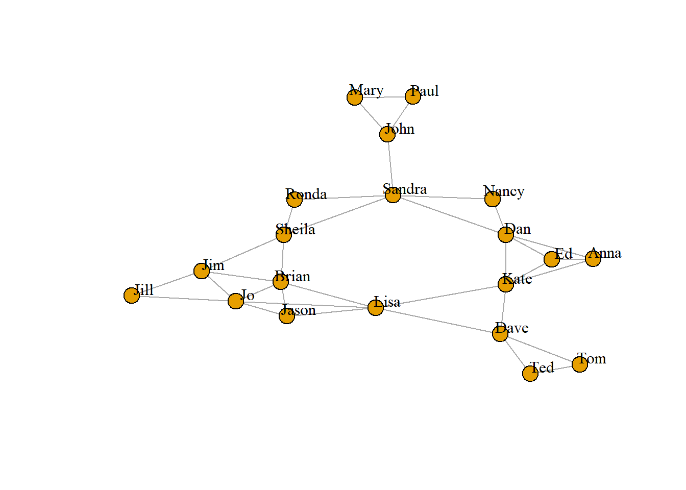

2.7 Selecting subgraphs

The preceding sections covered the basic information needed to create, read and manage network data objects in R. However, the data managements tasks for network analysis do not end there. There are any number of network analytic challenges that will require more sophisticated data management and transformation techniques.

In the rest two such examples are covered: preparing subsets of network data for analysis by filtering on node and edge characteristics, and turning directed networks into non-directed networks.

2.7.1 filtering based on node values

If a network object contains node characteristics, stored as vertex attributes, this information can be used to select a new subnetwork for analysis. In our example about news above, we have information about the type of media and audience size.

V(net)

+ 17/17 vertices, named, from 2ee6cb2:
 [1] s01 s02 s03 s04 s05 s06 s07 s08 s09 s10 s11 s12 s13 s14 s15 s16 s17

Suppose that we are only interested in relations between newspapers. Using the induced.subgraph command it is easy to select a subset of vertices and their relations. Note that we could als have used other attributes, such as audience size (should we be interested in larger organzations for instance).

news<-induced.subgraph(net, vids=which(V(net)$media.type==1))
plot(news,vertex.size=8, vertex.label = V(news)$media, edge.arrow.size=0.2)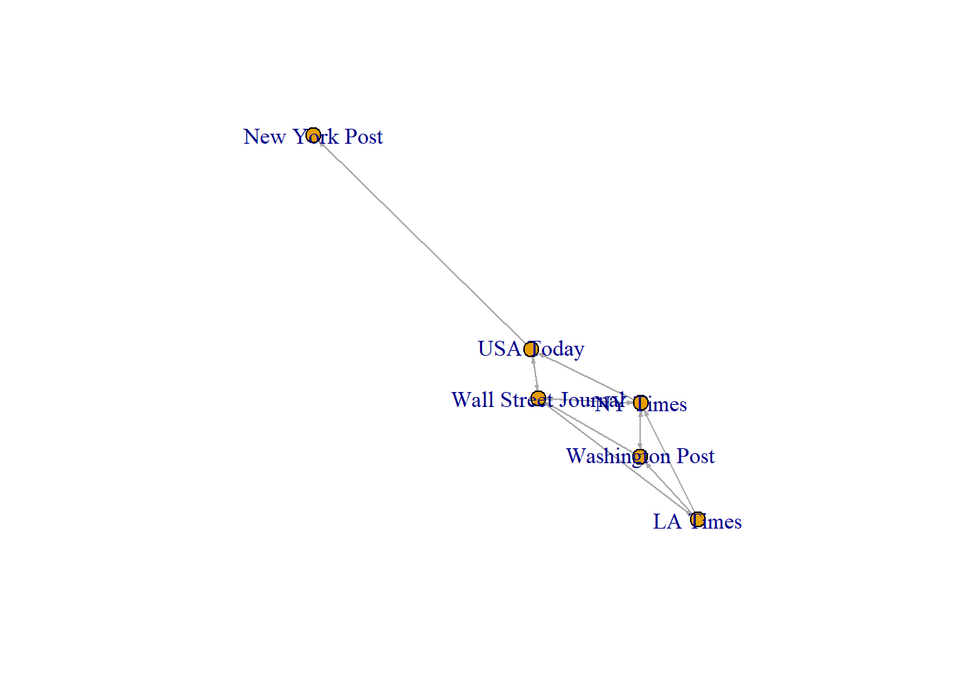

news

IGRAPH 2fa3c9b DNW- 6 12 -- 
+ attr: name (v/c), media (v/c), media.type (v/n), type.label (v/c),
| audience.size (v/n), weight (e/n), type (e/c)
+ edges from 2fa3c9b (vertex names):
 [1] s01->s02 s01->s03 s01->s04 s02->s01 s02->s03 s03->s01 s03->s04 s03->s05
 [9] s04->s03 s04->s06 s05->s01 s05->s02

Note that for the plot of the subgraph, we use the attributes of the subgraph as well (not the original)

2.7.2 Filtering Based on Edge Values

Selecting edges is less common, but can be useful. In Igraph the procedure is a bit different, since the “subgraph.edges” is used. It should include a sequence of edge ids. In the code below first a a vector d is created consisting of logical statements (TRUE if the weight attribute is larger than 10 or else FALSE). The v vector

d=E(net)$weight>10
d

 [1] FALSE  TRUE  TRUE  TRUE  TRUE  TRUE FALSE FALSE  TRUE  TRUE FALSE FALSE
[13] FALSE FALSE FALSE  TRUE FALSE  TRUE FALSE FALSE FALSE  TRUE FALSE  TRUE
[25]  TRUE  TRUE FALSE  TRUE  TRUE FALSE FALSE  TRUE  TRUE  TRUE FALSE FALSE
[37]  TRUE  TRUE  TRUE FALSE FALSE  TRUE  TRUE FALSE FALSE  TRUE  TRUE FALSE

The v vector is a count that runs from 1 to the number of edges (which is counted by the ecount command). The vector g contains those edge ids that have a weight larger than 10.

v <- rep(1:ecount(net))
g<-v[d==TRUE] #is edge > 10
net3 <- subgraph.edges(net, g, delete.vertices = TRUE)
net3

IGRAPH 2fcf9ee DNW- 17 25 -- 
+ attr: name (v/c), media (v/c), media.type (v/n), type.label (v/c),
| audience.size (v/n), weight (e/n), type (e/c)
+ edges from 2fcf9ee (vertex names):
 [1] s01->s03 s01->s04 s01->s15 s02->s01 s02->s03 s03->s01 s03->s04 s04->s03
 [9] s04->s11 s05->s02 s05->s15 s06->s16 s06->s17 s07->s08 s07->s10 s08->s07
[17] s08->s09 s09->s10 s12->s13 s12->s14 s13->s12 s14->s13 s15->s01 s16->s06
[25] s16->s17

2.7.3 removing isolates

A common filtering task with networks is to examine the network after removing all the isolates (i.e., nodes with degree of 0).

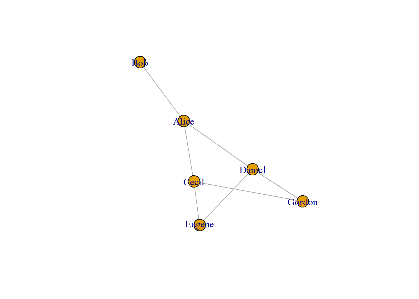
To illustrate we use the first organizational network collected, consisting of observational data on 14 Western Electric (Hawthorne Plant) employees from the bank wiring room first presented in Roethlisberger & Dickson (1939).

The employees worked in a single room and include two inspectors (I1 and I3), three solderers (S1, S2 and S3), and nine wiremen or assemblers (W1 to W9). There were five interaction categories, we focus on participation in arguments about open windows.

Initial.matrix <- read.csv("data/RDCON.csv", header=TRUE, row.names=1, check.names=FALSE, na.strings = "")
matrix <- as.matrix(Initial.matrix) 
RDCON <- graph.adjacency(matrix, mode="undirected", weighted=NULL)
plot(RDCON, asp=0.6)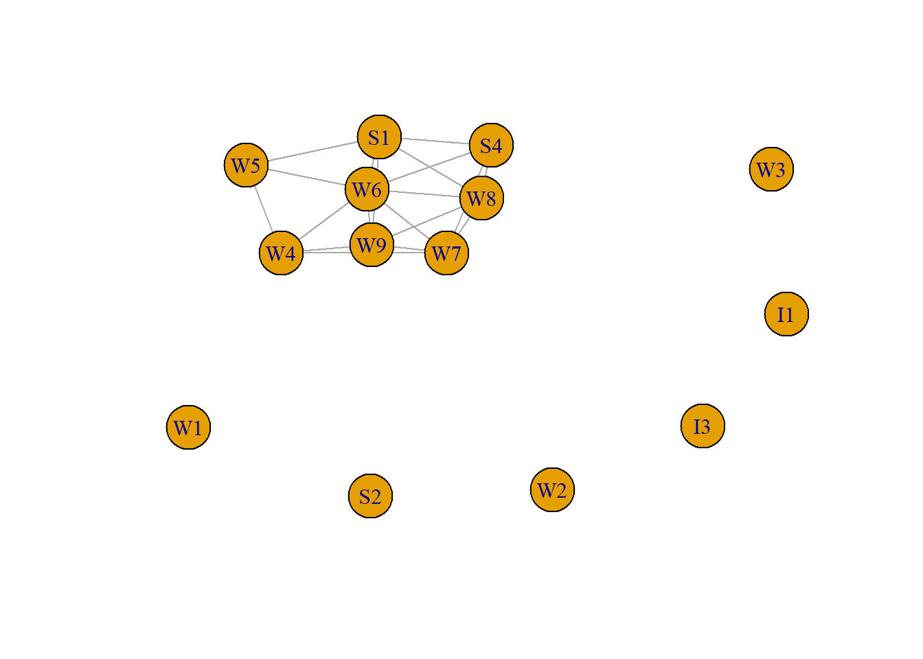

The first method is to simply find all the vertices without a connection (degree = 0), and remove them.

d <- degree(RDCON)
de <- delete.vertices(RDCON, (d==0)) 

The second method is to first detect the main component (connected subgraph), and select this component. Downside is that there maybe more components that may also be of interest, so use this only in case you are only interested in the main component.

m <- components(RDCON)
m<-unlist(m$membership)
Main_component_RDCON <- induced.subgraph(RDCON, vids=which(m==1))

2.8 Exercise part one

We will discuss these exercises in the next meeting, you dont have to hand them in.

1. Create a graph of your core network, and plot that network. Include relations between your contacts. You can use abbreviations for the names.

2. Add additional information (age or gender) to the igraph object.

3. What is the density of your core network? Density captures how many edges there are in a network divided by the total possible number of edges. In an undirected network of size N, there will be (N * (N-1))/2 possible edges. If you think back to the matrix underlying each network, N * N-1 refers to the number of rows (respondents) times the number of columns (respondents again) minus 1 so that the diagonal (i.e. ties to oneself) are excluded. We divide that number by 2 in the case of an undirected network only to account for that fact that the network is symmetrical.

4. Enter the “attiro.csv” network into R and create an Igraph object.

5. Are there multiple relations and self-loops? If so, Which relations and/or loops?

6. Are there isolates? If so, remove this/these isolate(s).

7. Consider the following edgelist (MM_edges1.csv) and nodes attributes (MM_Nodes.csv). This network concerns the diffusion of a new mathematics method in the 1950s. The diffusion process was successful since the new method was adopted in a relatively short period by most schools. The example traces the diffusion of the modern math method among school systems which combine elementary and secondary programs in Allegheny County (Pennsylvania, USA). All school superintendents who were at least two years in office were interviewed. They are the gatekeepers to educational innovation because they are in the position to make the final decision. The superintendents were asked to indicate their friendship ties with other superintendents in the county with the following question: Among the chief school administrators in Allegheny County, who are your three best friends? The year of adoption by a superintendent’s school is coded in the partition ModMath_adoption.clu: 1958 is class (time) one, 1959 is class (time) two, etc. Enter the data in R. Plot the network.

8. Select the early adopters (first two years), plot this subgraph.